Why Can't Claude Compute the Weather?

In this post, I want to talk about what actually happens when you ask an AI like Claude or GPT to compute the weather, and about PINO (Physics-Informed Neural Operator), an approach that emerged to tackle physics problems where data is scarce.

Looking around these days, quite a few people seem to treat LLMs like Claude or GPT as an all-purpose tool. And in a world where AI writes code, summarizes papers, and reviews contracts, it’s not hard to see why. I spend a good chunk of my day working alongside these AIs too, and I can definitely feel how much better they’ve gotten compared to before.

But there’s a catch. If we ask an LLM to “compute how the temperature in Seoul will change tomorrow,” it doesn’t actually solve the equations for how the atmosphere’s temperature and pressure will evolve. Instead, it produces a plausible-sounding sentence that looks like the result of a computation.

That’s because an LLM is a model that learned language by reading an enormous amount of text, not a model that learned by watching the Earth’s atmosphere move.

To be fair, models built on the same Transformer architecture as Claude are already posting results in weather forecasting that rival traditional numerical weather prediction. But those models were trained on decades of records of the Earth’s atmosphere, and a field like weather, where training data is plentiful, is actually closer to the exception.

Most physics problems, like the airflow around a car or the plasma inside a fusion reactor, have nowhere near enough data to train on. What these problems do have is one crucial thing going for them: we already know the equations that govern the phenomenon.

So in this post, I’ll start from why LLMs can’t compute the weather, then introduce PINO, an approach that learns by scoring itself against physics equations instead of answer data, and walk through how it actually works.

What Transformers Are Good At, and What They Aren’t

To talk about PINO, we first need to cover what the Transformer is, the neural network architecture that Claude and GPT have in common, and the real reason Claude can’t compute the weather.

What Claude and GPT Have in Common

The AIs we use all the time, like Claude, GPT, and Gemini, are usually grouped together as LLMs (Large Language Models). As the name says, they’re models that read an enormous amount of text and learned how to handle language.

These models come from different companies and vary in capability, but in fact most of today’s LLMs are built on the same blueprint, called the Transformer. It’s an architecture published by Google researchers in 2017, and its trace is already visible in the name GPT (Generative Pre-trained Transformer).

To borrow an analogy developers will find familiar, the Transformer is closer to a framework, and Claude or GPT is closer to an app built with that framework. Just as Toss (a Korean fintech app) and Netflix are completely different services even though both are built with React, each company’s model differs in the data it was trained on and its detailed design, even though they’re all based on the same Transformer. Of course, since each company modifies the Transformer in its own way, the relationship isn’t as clean-cut as a framework, but they’re similar in that they share the same skeleton.

So when we look at why Claude can’t compute the weather, we need to separate two cases: asking a conversational AI to do a physics calculation directly, and training the Transformer blueprint itself on physics data. I’ll come back to this distinction later. First, let’s see how the Transformer works.

Attention, an Operation That Compares Every Word Against Every Other

LLMs do so many things for us that they feel almost omnipotent, but if you sum up how they produce answers in a single sentence, it comes down to looking at the text so far and predicting the next piece of a word. These word pieces are called “tokens.”

For example, a word like “unbelievable” gets split inside the model into a few pieces like “un”, “believ”, and “able”, and each piece is turned into an array of numbers. The model looks at this sequence of arrays and probabilistically picks what the next piece will be.

This is also related to why Claude’s answers trickle out bit by bit when we chat with it. The model doesn’t build the whole answer in advance. It picks one token, looks again at the text with that token appended, picks the next token, and builds up the answer that way. So instead of making the user wait until the answer is fully done, showing it as it’s being produced is far less frustrating from the user’s side.

But to pick the next piece well, the model first has to properly understand the text so far. Say we’re choosing what comes after “I bought an apple yesterday, and it was so”. To come up with words like “sweet” or “expensive”, you need to know that “it” refers to the apple. The problem is that the token “it” by itself carries no information at all. In the end, a word’s meaning is determined by its relationships with the words around it.

So before picking the next token, the Transformer lets each token look around at the other tokens in the text, pull in the information it needs, and rewrite its own array of numbers. “It” pulls information from “apple” and turns into an array that carries the meaning “the it that refers to the apple.” This process of tokens exchanging information with each other is attention, the core of the Transformer blueprint. After repeating this process across many layers, the context of the entire preceding text is baked into the last token’s array, and the model looks at that array to pick the next token.

Written as a formula, attention looks like this.

There are a lot of symbols attached, but what it does is simple. Imagine the tokens in the text each sitting in a meeting room, one per seat. Each of them holds three things: a query $Q$ that says “here’s the information I need to pin down my meaning,” a key $K$ that says “here’s the information I have,” and a value $V$ that it can actually hand over. If you think of looking up a key with a query in a database and pulling out the value, the names should click right away. In the earlier example, the query of “it” holds “what am I referring to?”, and the key of “apple” holds “I’m something you can eat.”

$QK^T$ is the process where everyone looks at everyone else’s key and scores “how helpful would that person be for my question?” The query of “it” and the key of “apple” match well, so they get a high score. softmax turns those scores into proportions that sum to 1, and finally each token pulls in everyone’s values according to those proportions and mixes them. So “it” mixes in mostly the value of “apple” and rewrites its own array. This is exactly what I meant earlier by “pulling information from other tokens.” You can think of dividing by $\sqrt{d}$ as just a device for keeping the size of the scores in a reasonable range.

Now let’s count the cost. If there are $N$ people in the meeting room, everyone has to look at everyone’s key once, so the scoring happens $N \times N$ times. (Strictly speaking, in models like Claude or GPT each token only looks at the keys of tokens before it. It can’t peek at the part that hasn’t been written yet, but the cost is still proportional to the square of the number of tokens) If a piece of text consists of 1,000 tokens, that’s a million scores, which is no big deal for today’s GPUs.

And this structure is a really good fit for language. Even if the thing “it” refers to is several sentences back, attention can look at every word at once regardless of distance. On top of that, since who references whom is computed fresh for every sentence, it naturally handles the flexibility of “it” referring to an apple in one sentence and a car in another. That’s a big part of why the Transformer became the standard for language models.

When You Ask Claude About the Weather

So what happens if you ask Claude, “Given this pressure pattern, compute how the temperature in Seoul will change tomorrow”? As we saw, what Claude does is ultimately pick the next token. So Claude doesn’t actually compute the atmosphere’s temperature and pressure. It generates sentences that look like the result of a computation.

What Claude learned from is an enormous amount of text written by people. There’s surely plenty of writing about the weather in there, but that’s a far cry from numerical data recording how the Earth’s atmosphere actually moved over time. Reading tens of thousands of weather articles doesn’t make you able to compute tomorrow’s weather.

Of course, if you ask Claude to write weather simulation code, it’ll write pretty convincing code. So to be precise, it’s less that Claude “can’t” compute the weather and more that it “doesn’t” compute it when you ask directly.

There’s one more problem here: a model that learned by looking at patterns has no guarantee of obeying the laws of physics. A language model produces plausible answers based on patterns it saw in its training data. In language, that level of plausibility is usually enough, and if it’s wrong, you can ask again or have a person check.

But in the physical world, there are strict rules called conservation laws, so you can’t compute things this way. The water or energy inside a region can go up or down, but the change has to exactly match the sum of what flowed in and out across the boundary plus sources like heat or rain.

A model that learned only from patterns doesn’t know these rules, though, so it can make water that never flowed in or out slowly disappear, or conjure up energy from nowhere bit by bit. What’s worse is that these small errors pile up over time. If you feed the 1-hour forecast back in as input to predict 2 hours ahead, then feed that back in to predict 3 hours ahead, and keep rolling it forward, errors that were invisible at first end up producing completely bogus weather a few days later. It’s a lot like photocopying a photocopy over and over until the text gets mushier and mushier.

This isn’t a problem unique to Claude. Every model that learns patterns from data carries it, and it’s also the problem PINO tackles head-on later in this post.

Some Transformers Are Good at Forecasting the Weather

Does that mean Transformers can’t predict the weather at all? Not at all. If anything, weather is a field where Transformers have been a big success.

Pangu-Weather, which Huawei researchers published in Nature in 2023, is a weather model built on the Transformer architecture, and it reported more accurate results than the numerical forecasts of the European Centre for Medium-Range Weather Forecasts (ECMWF) on key metrics, including 5-day forecasts. Even ECMWF, which ran those numerical forecasts, put AIFS, a Transformer-based AI forecasting model, into actual operation starting in February 2025.

Of course, they didn’t just take a language model and use it as-is. They reworked it quite a bit to fit weather data. Predicting the weather means computing how values like the atmosphere’s temperature, pressure, and wind change over time, and these values aren’t chopped into discrete pieces like word tokens. For example, the temperature between Seoul and Pangyo, a city just south of it, doesn’t suddenly change at some point. It flows smoothly as a continuous value. Moving from Seoul to Pangyo doesn’t mean the temperature is 20 degrees one moment and then, ta-da, 19 degrees the next.

The problem is that computers are digital and can’t handle these continuous values as-is. A value being continuous is the same as saying there are infinitely many values between 0 and 1, and a computer can’t perform that kind of infinite computation.

So when computing the weather on a computer, we chop space into a fine grid and store a value in each cell. ERA5, one of the most widely used datasets in meteorology, divides the Earth into 1,440 cells horizontally and 721 cells vertically, which alone comes to about 1.04 million cells for a single point in time.

If you treated each of these cells as a token and applied attention, it’d be like a meeting room with 1.04 million people where everyone checks everyone’s key, and the scoring for a single point in time alone would come to about 1 trillion operations.

And that’s just for one variable at one altitude. Throw in all the altitudes and variables, and you’re in the sorry situation where no number of GPUs is enough. So models that use Transformers for weather cut costs by bundling several cells into a chunk and using that as one token, or by applying attention only between nearby cells.

Besides cost, resolution is another headache. When the resolution, meaning the number of cells the Earth is divided into, changes, the rules the model learned can fall out of alignment.

Transformers that handle grid data usually attach a cell index, something like “which position am I,” to each token, and based on that index they learn relationships like “reference the cell right next to you this much, and the cell three away this much.”

But think about it carefully. The “cell right next to you” learned on a 64x64 grid was some number of kilometers away in real distance, while on a 256x256 grid that same “cell right next to you” is only a quarter of that distance. In other words, even when showing the same weather, if the way you divide the cells changes, the learned rules fall out of alignment, so you need to apply separate corrections or retrain the model. This is less a problem with attention itself and more a problem with representing position by cell index, and there are techniques that compensate for it, but either way it’s something any model handling grid data has to worry about.

The real secret to why these models predict the weather so well lies elsewhere, though. It’s the data. ERA5, which I mentioned earlier, is a dataset in which ECMWF gathered past observation records and reconstructed the state of the Earth’s atmosphere on an hourly basis, and it now covers 1940 to the present. Both the Transformer-based Pangu-Weather and Google DeepMind’s GraphCast, which uses a different architecture called a graph neural network, were trained on 39 years of it, from 1979 to 2017. They essentially learned by watching, wholesale, how the Earth’s atmosphere moved every hour for 39 years.

What About Problems Without Data?

The problem is that a field like weather, with decades of records neatly piled up, is actually the exception.

For the airflow around a car that was just designed, there can’t be any observation records, since the car hasn’t even come into the world yet. Plasma inside a fusion reactor is hard to measure in the first place, and so is how bacteria move inside a thin tube placed in the body. In the end, if you need training data, you have to make it yourself by running a simulator thousands of times, and I’ll come back later to how painful that is.

What these problems do have instead of data is one thing to lean on: the equations that govern the phenomenon. How air flows and how heat spreads have been written down as equations for nearly 200 years. So instead of showing the model a pile of answer data, why not teach it those equations? The answer to that question is the star of this post, PINO.

What Problem Does PINO Solve?

So what would a tool look like that fits problems where data is scarce but the equations are known? Before taking PINO’s principles apart, let’s first look at what PINO ends up doing for you.

For example, when you want to know the airflow around a car body, you run a physics simulator, a program that honestly computes the laws of physics one step at a time. This program is accurate but slow, so evaluating a single design can take anywhere from a few hours to a few days. If you have to wait days every time you tweak the shape of the car body a little, the number of designs you can try computing is bound to be pretty limited.

PINO is a neural network that mimics this kind of simulator. Once trained, when you feed it new conditions, it approximates the result hundreds of times faster than the simulator, and in some cases close to a million times faster. Hearing just this much, you might think, “Isn’t that just a neural network trained on simulation results?” but PINO has a few more unusual properties.

First, it needs little training data. At the extreme, it can learn with no answer data at all, as long as you tell it the laws of physics.

Second, it directly scores how well the model’s answers obey the laws of physics during training. So rather than answers that merely look plausible, it moves toward answers that make physical sense.

Third, it works regardless of resolution. Give a model trained on a coarse grid a much finer grid, and it still makes predictions as-is. It doesn’t have the problem of being tied to cell indices that we saw earlier.

A real example makes this easier to grasp. Caltech researchers used Neural Operator technology, the foundation of PINO, to redesign a catheter, a thin tube used in hospitals.

When a catheter stays in the body for a long time, bacteria can swim up the tube and cause infections. Taking a cue from how bacteria swim, the researchers came up with the idea that putting triangular bumps shaped like shark fins on the inner wall of the tube would make it harder for bacteria to swim upstream.

The problem is that figuring out the most effective size, height, and spacing for the bumps means running simulations for countless shapes. The researchers built a neural network that, given a bump shape, predicts how bacteria will spread inside the tube, and used it to refine the bump shape. When they tested 3D-printed prototypes, they reported that 10 to more than 100 times fewer bacteria made it upstream compared to a smooth tube.

How is this possible? To answer that, we need to break the name PINO into a few pieces. In this post, I’ll follow these four questions in order.

1. Why are physics simulations slow in the first place?
2. How can you build a neural network that works regardless of resolution?
3. Why do you need the Fourier transform for that?
4. How can you score answers without answer data?

In this section, I’ll cover the first two questions, and then work through the Fourier transform and the scoring method one at a time in the sections that follow.

Why Are Physics Simulations Slow?

If you’ve ever done game development, you’re probably familiar with a physics engine’s update function. Every frame, it takes “the current state,” computes “the state after a very short amount of time,” and repeats this 60 times a second. A ball falling and a character jumping are all just repetitions of these small updates.

Physics simulations are essentially the same. The difference is that instead of one ball, you run update on every cell in space. Physicists write this update rule down as a formula, and that kind of formula is called a partial differential equation. The name sounds intimidating, but it’s enough to understand it as “a rule describing how each cell’s value changes over one frame.”

The simplest example is the rule for how heat spreads. Heat the middle of an iron rod with a lighter and then take it away, and the hot part gradually cools while the surroundings warm up, until eventually the whole rod reaches an even temperature. Written as a formula, it looks like this.

In this formula, $u$ is temperature, $t$ is time, and $x$ is the position along the rod. So the left side means “how fast is this cell’s temperature changing right now,” and $\frac{\partial^2 u}{\partial x^2}$ on the right side means “how much hotter, on average, are the cells on either side than this cell.” $\alpha$ is a material constant that’s large for materials that conduct heat well, like copper, and small for materials that don’t, like wood.

Put into words, this formula is saying something completely obvious: “a cell whose neighbors are hotter warms up, and a cell whose neighbors are colder cools down.”

And to put it in terms developers are familiar with, this is similar to an image blur filter. Blur is an operation that nudges each pixel toward the average of its surrounding pixels, so if you apply blur over and over, the image gets mushier and mushier until it eventually converges to the average value and becomes unrecognizable. Heat spreading is actually the exact same operation.

Since it’s hard to grasp from the formula alone, let’s move it into code. I’ve handed off the small array chores to es-toolkit functions like range and zipWith.

import { range, zipWith } from 'es-toolkit';

type Samples = number[];

const neighborPull = (temperatures: Samples, cellSize: number): Samples =>
  temperatures.map((center, cell) => {
    const left = temperatures[(cell - 1 + temperatures.length) % temperatures.length];
    const right = temperatures[(cell + 1) % temperatures.length];
    return (left - 2 * center + right) / (cellSize * cellSize);
  });

const heatStep = (temperatures: Samples, alpha: number, timeStep: number, cellSize: number): Samples =>
  zipWith(temperatures, neighborPull(temperatures, cellSize), (value, pull) => value + alpha * pull * timeStep);

const simulateHeat = (initial: Samples, alpha: number, timeStep: number, cellSize: number, steps: number) =>
  range(steps).reduce((temperatures) => heatStep(temperatures, alpha, timeStep, cellSize), initial);

Samples is an array of temperature values measured and recorded at each cell along the rod. neighborPull computes how much the cells on either side pull on this cell. (left - 2 * center + right) is shorthand for (left - center) + (right - center), so it comes out positive if the neighbors are hotter and negative if they’re colder.

heatStep is a one-frame update that nudges the temperature by the amount of the pull, and simulateHeat repeats it steps times. Here I’ve assumed the two ends of the rod are joined into a ring.

The formula looked terrifying, but once it’s in code, all it does is add and subtract a measly three neighboring values. So if the computation is this simple, why does weather prediction need a supercomputer?

The first reason is that you can’t make timeStep, the time interval of a single frame, as large as you’d like. In games, too, if frames are computed too far apart, you get bugs where a fast bullet passes right through a wall, and physics simulations are similar.

If you make timeStep too large in this code, the values of neighboring cells start bouncing up and down in alternation, the swings grow every frame, and eventually they get so large that the whole thing blows up. To run it stably, you need to satisfy roughly the following condition.

$\Delta t$ is timeStep in the code, and $\Delta x$ is cellSize. The key point is that $\Delta x$ appears squared on the right side, which means that if you split cells to half their size, you have to cut the time interval to a quarter. The number of cells doubles and the number of frames quadruples, so the total computation goes up 8 times. The more precisely you try to look, the more steeply the cost climbs.

The second reason is that real physics is far more complicated than heat spreading. Airflow is three-dimensional, and as wind carries wind along, small eddies and large eddies influence each other. To see this properly, you need very small cells and very short time intervals, which is how you end up in the tear-jerking situation of waiting days to check a single design.

In other words, physics simulations are slow not because we don’t know the rules. We know the one-frame rule exactly, but that simple rule has to be repeated an enormous number of times at a very fine granularity. So couldn’t we have a neural network learn a shortcut that skips all this repetition, where you put in the initial state and the final state comes right out? This is where we move on to the second question.

A Neural Network That Works Regardless of Resolution

The neural networks we usually know are, simply put, functions that take a fixed-length array of numbers and return an array of numbers. An image classification model takes a 224x224 array of pixels and returns an array with one probability per class, like “cat 0.9, dog 0.08, fox 0.02.” The key point is that the size of the input is baked into the model’s design.

What a Neural Operator wants to do is a bit different. Comparing them as TypeScript types makes the difference clear.

// A typical neural network

type NeuralNetwork = (input: number[]) => number[];

// Neural Operator

type Field = (position: number) => number;
type NeuralOperator = (input: Field) => Field;

While NeuralNetwork takes an array, NeuralOperator takes a Field, “a function that tells you the value at a position when you give it the position,” and returns another Field. For heat spreading, the input is “the initial temperature distribution” and the output is “the temperature distribution 10 seconds later.” If the earlier Samples is an array of temperatures measured and recorded at each cell along the rod, you can think of Field as the temperature distribution itself, before any measuring. Reading values at regular intervals from a continuous distribution like this to make an array is called sampling. (I covered sampling in detail using sound as the example in an earlier post, How Do Computers Hear Sound?)

In math, something that takes a function and returns a function is called an operator. You can think of it as the math version of what developers usually call a higher-order function. So the name Neural Operator ultimately means “a neural network that learns a higher-order function.” That means you can use the same neural network whether you sample the input temperature distribution into 64 cells or 256 cells, and how many cells to sample the result into is up to whoever is using it.

To use an analogy frontend developers will know, it’s similar to the difference between PNG and SVG. PNG represents an image as pixels, so it breaks up when you zoom in, while SVG stores rules like “draw a curve from here to there,” so it’s sharp at any size, regardless of resolution. In the end, you can think of a Neural Operator as wanting to treat physical phenomena like SVG rather than PNG.

Of course, since actual training still happens on data sitting on a grid, the analogy isn’t a perfect fit, but the direction of “learning the underlying rule rather than a specific resolution” is quite similar.

Why is this a natural goal? Think back to the heat-spreading rule we saw earlier. The rule “if the neighbors are hotter, you warm up” is the same whether you divide the rod into 10 cells or 1,000 cells. The rule itself has no concept of resolution. So it makes sense that a model that learned that rule should also work regardless of resolution.

But that’s easier said than done. A neural network is ultimately a machine that multiplies and adds arrays of numbers, so how on earth do you make it apply the same rule regardless of array size? This is where the Fourier transform comes in.

Seeing the World as a Sum of Sine Waves With the Fourier Transform

The Fourier transform, the star of the third question, is also the F in FNO (Fourier Neural Operator), the foundation of PINO. That makes it the most important ingredient in this post. Here, let’s first look at what the Fourier transform does, and then follow what happens when we look at heat spreading again through the lens of the Fourier transform.

Getting a Spectrum From a Waveform

Picture the equalizer in a music app. On screen, bars from bass to treble bounce up and down, with a row of sliders beneath them. Raise the bass slider and the thumping bass gets stronger; lower the treble slider and the sound gets muffled. But if you think about it, it’s strange. The sound coming out of the speaker is ultimately just one wiggly wave of vibrating air, so how can you pick out just the bass from it and boost it?

This is where the Fourier transform comes in. In the early 19th century, the French mathematician Joseph Fourier proposed the idea that any waveform, no matter how complicated, can be expressed as simple sine waves stacked on top of each other. Interestingly, the reason Fourier came up with this idea was precisely to solve the heat-spreading rule we saw earlier.

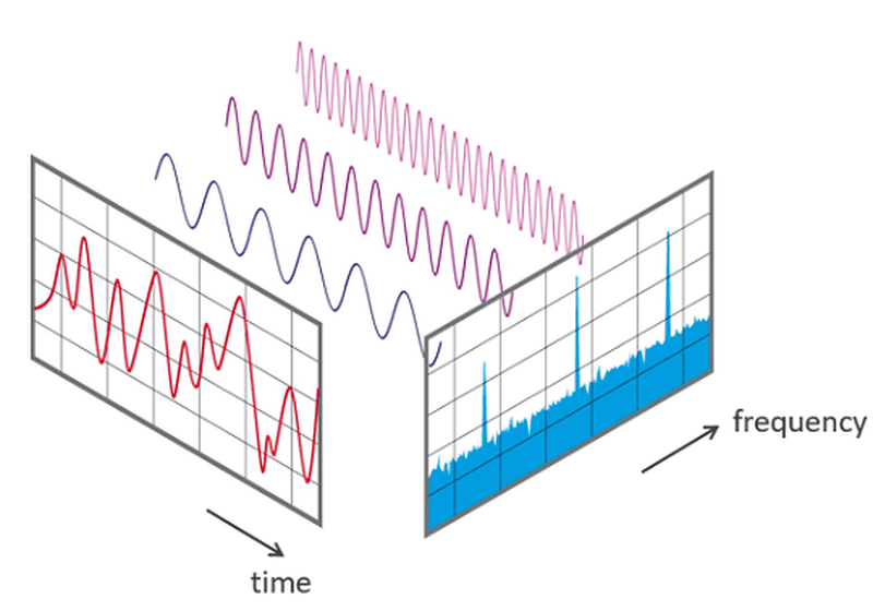The core of the Fourier transform is that any waveform in the world can be expressed as a stack of simple sine waves

The left side of the figure is the wiggly waveform we actually see, the middle is the sine waves that make up that waveform, and the right is a bar graph showing how much of each sine wave is mixed in. The Fourier transform is the tool that extracts the right side from the left, and the bar graph on the equalizer screen is exactly this result. This bar graph is called the frequency spectrum, or spectrum for short. The inverse transform goes the other way, looking at the spectrum and restoring the original waveform exactly.

As the figure shows, what distinguishes the sine waves from each other is how densely they oscillate. In this post, treating the whole signal as a single interval, I’ll call the number of times a sine wave oscillates over that interval $k$. This count is the frequency, and a sine wave with small $k$ is called low-frequency while one with large $k$ is called high-frequency. In music terms, low-frequency is bass and high-frequency is treble.

The formula for getting the spectrum looks like this.

There are several symbols, so let’s take them apart one by one. Starting with the ingredients, $u_n$ is the value of the original signal at cell $n$, and $N$ is the total number of cells.

$\sum$ means to vary $n$ from 0 to the end and add everything up. In code, it’s the same as computing a total with reduce, and the code below uses es-toolkit’s sumBy, which does that in one go. sumBy(array, fn) applies the function to each element of the array and adds up all the results.

$\cos\left(2\pi \frac{kn}{N}\right)$ is the value at cell $n$ of a reference sine wave that oscillates $k$ times over the whole interval. The part in parentheses looks complicated, but you can think of it as just a device tuned so that it oscillates exactly $k$ times over $N$ cells.

Splitting the computation into two lines, cosine and sine, like $a_k$ and $b_k$, is for recording not only the strength of the sine wave but also how far it’s shifted sideways, but for this post it’s enough to care only about strength.

So what this formula does is “multiply the signal and the reference sine wave cell by cell and add everything up.” If the signal contains a lot of that sine wave, their peaks and troughs line up well and the sum gets large; if not, the positives and negatives cancel out and it gets close to 0. It’s pattern matching: holding up each reference sine wave one at a time and measuring how well it lines up.

import { sumBy } from 'es-toolkit';

type Component = { cosine: number; sine: number };

const waveAngle = (index: number, cell: number, cellCount: number) => (2 * Math.PI * index * cell) / cellCount;

const toComponents = (signal: Samples): Component[] => {
  const cellCount = signal.length;
  return range(cellCount / 2 + 1).map((index) => ({
    cosine: sumBy(signal, (value, cell) => value * Math.cos(waveAngle(index, cell, cellCount))),
    sine: -sumBy(signal, (value, cell) => value * Math.sin(waveAngle(index, cell, cellCount))),
  }));
};

const fromComponents = (components: Component[]): Samples => {
  const cellCount = (components.length - 1) * 2;
  const weight = (index: number) => (index === 0 || index === components.length - 1 ? 1 : 2);
  return range(cellCount).map(
    (cell) =>
      sumBy(components, ({ cosine, sine }, index) => {
        const angle = waveAngle(index, cell, cellCount);
        return weight(index) * (cosine * Math.cos(angle) - sine * Math.sin(angle));
      }) / cellCount,
  );
};

toComponents is the function that gets the spectrum, and fromComponents is the function that combines the spectrum back into a waveform. cosine and sine in Component correspond to $a_k$ and $b_k$ in the formula, and the formula’s $k$ became index, $n$ became cell, and $N$ became cellCount. The formula’s $\sum$ just became sumBy, and it’s a double loop that sweeps the entire signal once for each cell of the spectrum.

One thing worth noticing is that toComponents only counts $k$ up to half the number of cells. Within a 64-cell signal, 32 is the maximum number of times a sine wave can oscillate, so there’s no need to look beyond that. In exchange, when fromComponents combines them back, it counts every sine wave except the very first and very last twice. Real FNO implementations use this kind of half spectrum too.

Let’s run an experiment. We’ll make a signal mixing a low-frequency sine wave that oscillates 3 times with a high-frequency sine wave that oscillates 10 times, and get its spectrum.

const cellCount = 64;
const grid = range(cellCount).map((cell) => (2 * Math.PI * cell) / cellCount);
const signal = grid.map((position) => Math.sin(3 * position) + 0.3 * Math.sin(10 * position));

const strengths = toComponents(signal).map(({ cosine, sine }) => Math.hypot(cosine, sine));

Math.sin(3 * position) is a sine wave that oscillates 3 times over the whole interval, and strengths holds how strong each sine wave is, for each cell of the spectrum.

Print out strengths and you’ll see values spike only at cells 3 and 10 while the rest are nearly 0. A signal that looked like a wiggly line to the eye turns, in the spectrum, into very simple information: “this much of sine wave 3, a little of sine wave 10.”

For the record, this toComponents is the simplest version I wrote for the sake of understanding, so it gets painfully slow as the number of cells grows. In practice, people use an algorithm called FFT (Fast Fourier Transform), which reuses intermediate computations to produce the same result much faster. With a million cells, my version does close to a trillion operations, while FFT gets it done in roughly 20 million, so the difference is huge.

But what do we gain from knowing the spectrum? This is where the single most important observation in this whole post comes in.

Blur Wipes Out High Frequencies First

Earlier, I said heat spreading is just like a blur filter. So when you apply blur to a photo, what disappears first? The sharp, fine details, like a single strand of hair or the edges of text. On the other hand, the big picture, like “the left side is bright and the right side is dark,” survives even after quite a few rounds of blur.

Explained again in terms of sine waves, you can understand blur as wiping out high frequencies quickly and low frequencies slowly. Exactly the same thing happens when heat spreads. If you actually apply the heat-spreading rule to the spectrum and solve it, the strength of each sine wave changes over time like this.

$\hat{u}_k(0)$ is the strength of sine wave $k$ in the initial spectrum, and $\hat{u}_k(t)$ is its strength after time $t$ has passed. The $e^{-\alpha k^2 t}$ multiplied in between is the fraction of sine wave $k$ that remains after time $t$. $e^{-\text{something}}$ is a value that’s 1 when “something” is 0 and gets closer to 0 as it grows. So this formula is saying “high-frequency waves that oscillate often disappear faster as time passes.”

The numbers make it more vivid. With $\alpha = 1$ and $t = 0.1$, about 90% of the low-frequency wave that oscillates once remains. Only about 8% of the sine wave that oscillates 5 times remains. The high-frequency wave that oscillates 10 times is down to 0.005%, so you can consider it effectively gone.

And when you move this formula into code, the simulation that earlier required the grunt work of running update thousands of times ends with a single multiplication on the spectrum.

const solveHeat = (initial: Samples, alpha: number, time: number): Samples =>
  fromComponents(
    toComponents(initial).map(({ cosine, sine }, index) => {
      const remaining = Math.exp(-alpha * index * index * time);
      return { cosine: cosine * remaining, sine: sine * remaining };
    }),
  );

Since the spectrum’s index is the formula’s $k$, all it does is get the spectrum, multiply each sine wave’s strength by the fraction that remains, and combine them back.

This is where it really sinks in that the Fourier transform was originally built to solve the heat-spreading problem. A problem that, viewed on the cells, requires endlessly repeating “compare with your neighbors and adjust a little,” turns into “adjust one slider per sine wave” when viewed on the spectrum. The same data can make a problem this much easier or harder depending on how you look at it.

So couldn’t we solve the weather this way too? Unfortunately, clean shortcuts like this only show up for rules as simple as heat spreading. In heat spreading, sine waves don’t interfere with each other and each fades at its own pace, so adjusting a separate slider for each sine wave is all it takes to get the right answer.

But complex problems like airflow are a different story. Because wind carries wind along, large eddies break apart and create small eddies, and small eddies gather and in turn influence the larger flow. Seen as a spectrum, low frequencies and high frequencies get thoroughly mixed together.

In problems like this, even if you know the one-frame rule exactly, you can’t derive a formula for the shortcut that jumps straight to the result of repeating it tens of thousands of times. That’s why you need a neural network that learns that shortcut from data.

Even so, the observations from heat spreading give us two important hints.

The first hint is that you can often throw away the high frequencies. There’s no need to carefully compute high frequencies that will vanish soon anyway. Handle a few low frequencies well, and you capture most of the information. The way JPEG compression shrinks photo file sizes works similarly.

JPEG converts a photo into frequency components and then boldly throws away the high-frequency information that the human eye barely notices. To the human eye, it all looks pretty much the same anyway. Of course, in problems where high frequencies matter, like turbulence where eddies keep breaking down into ever smaller ones, this becomes a weakness and can be the reason predictions come out blurry.

The second hint is that the sliders are attached to sine waves, not cells. Whether you sample a signal into 64 cells or 256 cells, a sine wave that oscillates 3 times is still a sine wave that oscillates 3 times. So a rule like “keep only 40% of sine wave 3” can be applied regardless of resolution.

This might sound familiar if, like me, you’ve done some audio work. Whether a file was recorded at 44.1kHz or 96kHz, an equalizer setting like “boost the 100Hz band by 3dB” applies exactly the same way. The sample rate is only a matter of how densely the sound was recorded; it doesn’t change the nature of the 100Hz sound itself.

These two hints are exactly where FNO starts.

Assembling the Ingredients Into a Neural Network

We’ve gathered all the ingredients, so now it’s time to assemble them. The assembly happens in two steps. First, we build FNO, which carries the two hints from heat spreading straight into a neural network architecture, and then we put the answer to the fourth question, checking the answer, on top of it to get PINO.

FNO, an Equalizer That Tunes Its Own Sliders

FNO, published in 2020 by Zongyi Li, Anima Anandkumar, and others at Caltech, is an architecture that carries the ideas so far straight into a neural network. To sum it up in one line, FNO is “an equalizer that learns its own slider positions.”

In the heat-spreading problem, we knew exactly where each sine wave’s slider should go from the remaining-fraction formula. In problems where sine waves mix with each other, like airflow or plasma, that value can’t be derived from a formula. So what do you do? You show the model lots of examples where putting in the initial state gives you the later state, and have it learn the slider positions. That’s the core idea of FNO.

Written as a formula, one layer looks like this.

It looks like a lot of symbols, but you already know all of them. $v_{\text{in}}(x)$ is the value at position $x$ among the values coming into the layer, and $v_{\text{out}}(x)$ is the value going out of the layer. $\mathcal{F}$ is getting the spectrum, and $\mathcal{F}^{-1}$ is combining the spectrum back. $R$ is the slider values to be learned. So the right-hand term inside the parentheses means: get the spectrum, adjust the strengths by the sliders, and combine them back.

The left-hand term $W v_{\text{in}}(x)$ is the part that slightly transforms each cell by looking only at its own value, and $\sigma$ is a nonlinear transformation called an activation function. Why are these two needed?

The $W$ term is a path that passes each cell’s original value straight through without going through the spectrum. Since the equalizer cuts off high frequencies, it tends to lose fine detail, and it’s enough to understand the $W$ term as making up for that lost information.

$\sigma$ is needed because there are things an equalizer alone can’t do. An equalizer only boosts or cuts the strength of each sine wave; it can’t turn sine wave 3 into sine wave 10. So applying an equalizer ten times in a row ends up the same as applying a single equalizer with different slider values, and stacking layers does nothing no matter how many you add.

But to solve problems like the airflow we saw earlier, where large eddies create small eddies, you need an operation where sine waves mix and give rise to new sine waves. That’s the role $\sigma$ plays. Here, we use its simplest form, “a function that turns negative values into 0.”

How does such a simple function mix sine waves? Take a single sine wave 1 and turn its negative part into 0, and you get a shape with its bottom shaved flat. That shape can no longer be represented by a single sine wave, so if you get its spectrum, you’ll find new sine waves like 2 and 4 that weren’t there originally. This is also why the next layer can recreate the high frequencies the equalizer cut off.

If you’ve roughly got the idea, let’s move the formula into code. First, the equalizer part.

const applyEqualizer = (signal: Samples, sliders: number[]): Samples =>
  fromComponents(
    toComponents(signal).map(({ cosine, sine }, index) => {
      const gain = sliders[index] ?? 0;
      return { cosine: cosine * gain, sine: sine * gain };
    }),
  );

This function looks almost identical to solveHeat, which we wrote above, except that instead of the remaining-fraction formula, it pulls values from the sliders array.

The length of the sliders array is the number of sine waves to keep. With only 12 sliders, only the low frequencies from 0 to 11 survive, and every higher frequency gets caught by ?? 0 and thrown away. The first hint, “you can throw away the high frequencies,” lives in this single line. Real FNO learns not only the strength but also how far to shift each sine wave sideways, but strength alone is enough to understand the principle.

Now that we have the equalizer, we can build one layer, and the whole model made by stacking multiple layers.

type FourierLayer = {
  sliders: number[];
  scale: number;
  bias: number;
};

const relu = (value: number) => Math.max(0, value);

const applyLayer = (input: Samples, { sliders, scale, bias }: FourierLayer): Samples =>
  zipWith(input, applyEqualizer(input, sliders), (value, equalized) => relu(scale * value + bias + equalized));

const fourierNeuralOperator = (layers: FourierLayer[]) => (input: Samples) =>
  layers.reduce(applyLayer, input);

The formula’s $W v_{\text{in}}(x)$ became scale * value + bias, the equalizer part became applyEqualizer, and $\sigma$ became relu.

Of course, real FNO is more complex, with dozens of channels per cell instead of a single number, but the core skeleton can be implemented with this much. The formula in the paper looked pretty terrifying, but once moved into code, it boils down to three simple steps: “get the spectrum, adjust a few low frequencies with sliders, and transform back.”

So what exactly does training do? It’s similar to how most AI models learn. You compute how far the model’s prediction is from the answer as a single number, then gradually adjust the sliders, scale, and bias values in the direction that makes that number smaller. This number is called the loss.

You can tell which direction to adjust by nudging a single value very slightly and seeing whether the loss goes up or down. Neural network libraries have a feature that automatically computes this direction for all values at once, and it’s called automatic differentiation. This feature will show up again later when we talk about the catheter example.

Let’s see how this architecture handles the problems with grid data we talked about earlier.

First, computation cost. Thanks to FFT, getting the spectrum and transforming back is fast, and the slider adjustment only needs to happen for the 12 sine waves we kept. (Real FNO has multiple channels, so it does a small matrix multiplication once per sine wave)

Next, field of view. Sine wave 1, which has the lowest frequency, oscillates once in a big sweep across the whole interval. Adjusting this sine wave’s strength is the same as mixing information from the whole interval all at once. So you can say FNO sees the entire space at once with just a single layer.

In that sense it resembles attention, which also sees every token at once. The difference is that attention computes “who references whom” fresh for every input, while FNO learns a fixed rule: “which sine waves to keep, and by how much.”

Finally, the most interesting part: resolution independence. Since the sliders are attached to sine waves rather than cells, the same sliders can be used as-is on a 64-cell input and on a 256-cell input. Let’s check it ourselves.

const sample = (field: Field, resolution: number): Samples =>
  range(resolution).map((cell) => field((2 * Math.PI * cell) / resolution));

const initialTemperature: Field = (position) => Math.exp(-4 * (position - Math.PI) ** 2);

const sliders = range(12).map((waves) => Math.exp(-0.05 * waves * waves));

const coarse = applyEqualizer(sample(initialTemperature, 64), sliders);
const fine = applyEqualizer(sample(initialTemperature, 256), sliders);

We sampled the same temperature distribution into 64 cells and 256 cells, then applied the same sliders to each. Instead of going through training here, I plugged the values from the earlier remaining-fraction formula with $\alpha t = 0.05$ directly into the sliders. If FNO were trained on heat-spreading data, ideally these are exactly the values it should find.

Compare coarse[cell] with fine[4 * cell] and you get the same values down to a dozen or so decimal places. That means sliders tuned on 64 cells produce the same result when used as-is on a 256-cell input. Of course, this compares only the equalizer part in isolation. Real FNO has nonlinear operations like relu between layers, so results shift a little when the resolution changes, and it’s not as if it discovers, at 256 cells, details that were never in the 64-cell data to begin with.

You might be thinking, “Well, of course, you sampled the same temperature distribution,” so let’s set up a control group too. This time, it’s a rule that defines relationships based on cell indices, as we discussed earlier.

const cellRule = (temperatures: Samples): Samples =>
  temperatures.map((value, cell) => {
    const left = temperatures[(cell - 1 + temperatures.length) % temperatures.length];
    const right = temperatures[(cell + 1) % temperatures.length];
    return 0.5 * value + 0.25 * (left + right);
  });

const applyTimes = (rule: (temperatures: Samples) => Samples, times: number, input: Samples) =>
  range(times).reduce((temperatures) => rule(temperatures), input);

const coarseCell = applyTimes(cellRule, 10, sample(initialTemperature, 64));
const fineCell = applyTimes(cellRule, 10, sample(initialTemperature, 256));

cellRule is a rule defined in units of cells: “mix half of your own value with a quarter each of the cells right next to you.” Apply this rule 10 times on 64 cells, and the highest temperature at the middle of the rod drops from 1 to about 0.85, but on 256 cells it stays nearly the same at about 0.99. Since “the cell right next to you” on 256 cells is actually only a quarter of the distance, applying the same rule spreads the heat far less. This is exactly why a model that learned relationships based on cell indices gets tied to resolution.

The FNO paper called this property zero-shot super-resolution. It showed experiments where a model trained at a coarse resolution was run as-is at a fine resolution it had never seen, and the follow-up PINO paper reported that accuracy didn’t drop even when the resolution was raised this way.

PINO, a Way to Score Without Answers

With FNO, we can build a model that’s fast and free from resolution constraints. But one problem remains: FNO still learns by looking at answers.

To train it, you need examples on the order of thousands saying “given these initial conditions, the result is this,” and who makes those answers? The same slow simulator I said earlier takes days.

Wait a minute. We’re building a neural network because simulation is slow, but to train that neural network we have to run the slow simulation over a thousand times. It’s a strange situation. On top of that, a model that just imitates examples still has no guarantee of obeying the laws of physics.

So couldn’t we score without answers?

Think back to math tests in school. If you solve $x^2 - 5x + 6 = 0$ and get $x = 2$, there’s a way to check whether you got it right even without an answer key. Just plug 2 back into the original equation. $4 - 10 + 6 = 0$, so it’s the right answer. That’s checking your answer.

This is exactly PINO’s idea. Earlier, we said we don’t know the shortcut for airflow, but we know the one-frame rule exactly. So we can plug the model’s prediction directly into that rule and add how much it violated the rule to the loss. For heat spreading, you look at the temperature change the model predicted and check, cell by cell, “did the cell whose neighbors are hotter really warm up by that much?” This scoring needs no answer data. All you need is the one-frame rule.

But there’s a trap here: a lazy answer that just puts 0 in every cell somehow passes the check too. If the temperature is 0 everywhere, the difference with the neighbors is 0 and the change is 0, so it obeys the rule perfectly.

This trap can be blocked with the initial state, though. The rule only tells you how the temperature changes, not where it starts. In the earlier simulateHeat, too, the rule heatStep alone didn’t determine the result. You needed initial, the starting value passed to reduce, for the result to be pinned down to one.

PINO is the same. Even if we don’t know the final result, we know the initial temperature distribution, because we put it in ourselves. So if we also score “does the start of the prediction match the initial state we gave it?”, the countless answers that obey the rule get narrowed down to the one that starts from the starting point we gave.

Written out in words, PINO’s loss looks like this.

The gap from the answer is a term that’s only scored when answer data exists, and the degree of rule violation is the newly added check term. $\lambda$ is a ratio that sets how much weight to give the check term. The formula in the actual PINO paper has the same structure, adding up several terms with weights attached.

Strictly speaking, checking the answer needs more than the result at a single point in time; you also have to see how the temperature changes as time flows. Real PINO treats time as a continuous function too and gets the rate of temperature change directly through differentiation, but moving all of that into code is too much hassle, so here let’s just say the model predicts temperature distributions at multiple points in time all at once and returns them as an array. I’ll call this array Trajectory, since it’s a trajectory.

import { meanBy, windowed } from 'es-toolkit';

type Trajectory = Samples[];

const meanSquare = (values: number[]) => meanBy(values, (value) => value * value);

const gap = (predicted: Samples, expected: Samples) =>
  meanSquare(zipWith(predicted, expected, (a, b) => a - b));

const lawViolation = (trajectory: Trajectory, alpha: number, timeStep: number, cellSize: number) =>
  meanSquare(
    windowed(trajectory, 2).flatMap(([current, next]) =>
      zipWith(current, next, neighborPull(current, cellSize), (now, later, pull) => (later - now) / timeStep - alpha * pull),
    ),
  );

gap is a function that measures how different two temperature distributions are. It squares the difference in each cell and takes the average, so that coming out too hot and coming out too cold count toward the loss equally.

lawViolation pairs up consecutive points in time, then for each cell computes the difference between “how fast the temperature actually changed” and “how fast it should have changed according to the rule.” The point is that neighborPull, which we used in the simulation, gets reused here as-is. The simulator used this rule to produce the next state, and PINO uses the same rule to examine the model’s answer. If the model obeyed the rule perfectly, this value is 0.

type LossInput = {
  prediction: Trajectory;
  initial: Samples;
  answer?: Samples;
  alpha: number;
  timeStep: number;
  cellSize: number;
  lambda: number;
};

const pinoLoss = ({ prediction, initial, answer, alpha, timeStep, cellSize, lambda }: LossInput) => {
  const startGap = gap(prediction[0], initial);
  const answerGap = answer ? gap(prediction[prediction.length - 1], answer) : 0;
  return startGap + answerGap + lambda * lawViolation(prediction, alpha, timeStep, cellSize);
};

Notice that initial is required while answer is an optional argument. We always know the initial state because we put it in ourselves, but the answer may or may not exist. If there’s an answer, it also looks at the gap from the answer; if not, it scores using only the initial state and the check. That’s exactly the flexibility PINO has.

The “needs little data” property I introduced earlier comes straight from this scoring method. You prepare just a small amount of expensive simulation answers at a coarse resolution, and do the checking at a much finer resolution. Since FNO is free from resolution constraints, you can mix the two.

At the extreme, it can learn with no answers at all, using only the initial state and the check, and the paper reported solving even flow problems with intricately tangled eddies this way. Of course, this method isn’t a silver bullet either. Reportedly, for the problem of predicting the same flow over a much longer time span, PINO couldn’t solve it properly without answer data.

The check is useful in practice too. When a never-before-seen problem comes in, you don’t know the answer, but you do know the rule, so after making a prediction you can refine the model a bit more for that one problem in the direction of “obeying the rule better.”

The idea of scoring with the laws of physics didn’t actually start with PINO. It became widely known through a method called PINN (Physics-Informed Neural Network), published in 2019, but PINN had to train a neural network from scratch every time it solved a single problem.

On top of that, training often didn’t go well in problems where low and high frequencies are intricately mixed, such as flows where large and small eddies are tangled together. That’s because neural networks naturally tend to learn low frequencies easily and struggle to learn high frequencies. PINO put this checking approach on top of FNO, so it learns a rule that solves a whole family of similar problems rather than just one. Once trained, it produces an answer in a single inference pass even when new conditions come in.

Now we can gather the answers to the original question, “How is this possible?” Simulations were slow because a simple one-frame rule has to be repeated at a very fine granularity. Seen on the spectrum, that repetition turns into slider adjustment, and since the sliders are attached to sine waves rather than cells, they don’t care about resolution. FNO is an architecture that learns from data the slider values that can’t be derived from a formula, and PINO attaches a check using the one-frame rule to it, so that it produces physically sensible answers even when answers are scarce.

Neural Operators in the Real World

Once you understand the principles, two things naturally make you curious: where it’s actually being used, and how much you can trust the results.

There’s one thing to point out up front. Many of the examples introduced here are FNO-family models trained only on simulation data, without the check. PINO is an extension that adds the check to FNO, so you can read the examples below as showing how the technology underlying PINO is being used in the real world.

Where Is It Being Used?

Having understood this much, you can roughly guess where this technology would be used. What they have in common is work that used to require running simulations for hours or days, and work that only becomes meaningful when repeated thousands of times.

The most prominent field is weather prediction. FourCastNet, which NVIDIA published in 2022, is a model that predicts global weather, and interestingly, it uses an architecture where the attention slot in a Transformer skeleton is replaced with an FNO-style Fourier operation. The paper reported generating a week’s worth of forecasts in under 2 seconds, several orders of magnitude faster than traditional numerical forecasting.

That said, this speed is the time for prediction alone with a model that has already finished training, so the cost of training isn’t included, and its accuracy was also a bit lower than ECMWF’s numerical forecasts at the time. And since this model too was trained on the decades of atmospheric records we talked about earlier, it reconfirms that weather is a data-rich field.

When prediction gets this fast, you can run hundreds or thousands of forecasts with slightly perturbed initial conditions and compute even the uncertainty, like “there’s a 70% chance the typhoon takes this path.” With traditional methods, cost limited this to a few dozen or so.

It’s also used in car and aircraft design. Predicting how air resistance changes with the shape of a car body has traditionally been the domain of slow simulations.

A model called GINO (Geometry-Informed Neural Operator), published by Caltech and NVIDIA researchers, takes complex 3D car body shapes and predicts the pressure on their surfaces, and it reported being about 26,000 times faster for drag computation than an existing GPU-optimized simulator. When the time to evaluate a single design shrinks this much, sweeping through thousands of candidates, rather than a few designs a person picked by intuition, becomes a realistic option.

The catheter example I introduced earlier goes in a slightly different direction, because it didn’t stop at making predictions fast but ran prediction in reverse.

In the FNO section, I said neural network libraries can automatically compute which direction the loss changes when you nudge a value slightly. Apply that same feature to the input instead of the model’s weights, and you can compute “which way should the size or spacing of the bumps change so fewer bacteria swim up?”, and the researchers actually refined the bump shape this way.

They flipped a tool for predicting outcomes into a tool for finding designs that produce the outcome you want. Traditional simulators do have techniques that trace things backward, like the adjoint method, but they have to be implemented separately for each simulator and are computationally heavy.

Beyond these, research is expanding into a wide range of fields: carbon storage research predicting how carbon dioxide buried underground will spread over decades, research predicting plasma changes inside a fusion reactor roughly a million times faster than traditional simulations, seismic wave propagation prediction, predicting warping during 3D printing, and digital twins that replicate factory equipment as real-time physical models.

So Is It a Silver Bullet?

By now, you might be thinking, “So PINO is the answer to physics simulation.” But just as LLMs like Claude aren’t all-powerful, PINO isn’t either. Every neural network architecture comes with both strengths and limitations.

PINO’s first limitation is that it doesn’t necessarily obey the laws of physics. PINO’s check term is just a value added to the loss, not a hard constraint. The model will of course learn in the direction that reduces the loss, but there’s no guarantee it will never violate the rules.

In other words, PINO is a model that “mostly obeys” the laws of physics, not one that “always obeys” them. Some articles introducing PINO give off the impression that it solves physics problems without error, but if you follow the principles, it’s more accurate to say it approximates them much faster than existing methods, with fairly small errors.

The second is a constraint of the Fourier transform itself. The basic Fourier transform assumes the signal repeats endlessly in the same shape, and it works well only when the cells are laid out on a neat, regular grid. But real cars and blood vessels have irregular shapes and don’t repeat. So follow-up research keeps coming out to compensate, such as methods that unfold complex shapes onto a regular grid or methods that handle the edges more accurately.

The third is that it’s weak in situations outside the range it learned. Ask a model that only learned from slow water flow about supersonic airflow, and it’ll have a hard time answering properly. This is actually a limitation of every machine learning model, Transformers included. So in practice, the more realistic use is to quickly filter thousands of candidates with a model like PINO, then carefully verify only the final few candidates with a traditional simulator.

And the relationship with Transformers isn’t black and white either. Earlier I said FNO sees the whole thing at once like attention, and in fact there’s been a lot of recent research redesigning attention within the Neural Operator framework.

In the end, I think the key isn’t whether it’s a Transformer or not, but how much data you have and how much of the rules you already know about the problem you can build into the model. If data is abundant, learn from the data; if data is scarce, teach it the rules you know.

Closing Thoughts

I started digging into this topic because of a simple question. These days everyone talks about LLMs as if they can do anything, but there’s no way they really can, right? So what can’t LLMs do, and where do those limits come from?

Following the thread, the answer turned out to be simpler than I expected: a model only knows as much as it has seen. Claude can’t compute the weather not because the Transformer architecture falls short, but because it has never seen the atmosphere, and the same Transformer, once it has seen decades of atmospheric records, can even predict the weather better than traditional numerical forecasting. In other words, the question “Can AI do this?” is really closer to “Has AI ever seen this?”

So what do you do about problems it has never seen? PINO’s answer was not to simply trust a plausible answer, but to check it against rules you already know. You may not have answer data, but you do know the equations, so you measure how much the model’s answer violates them and pull it toward answers that make physical sense.

I actually think this isn’t so different from what developers deal with every day working with LLMs. An LLM has never seen our service’s codebase or domain rules, so in those areas it has no choice but to produce code that merely looks plausible.

So what matters is less agonizing over whether to trust an LLM’s answer, and more building a structure where you can check that answer with types, tests, and domain rules, the way PINO scores itself with equations. And in the end, I believe making AI work properly where data is scarce is the job of the people who know the rules of that problem.

And with that, I’ll bring this post on why Claude can’t compute the weather to a close.