[Simulating Celestial Bodies with JavaScript] Implementing Planetary Motion
Implementing a celestial simulation using Kepler's equation
![[Simulating Celestial Bodies with JavaScript] Implementing Planetary Motion](/static/746a090a9954b09cea8d75079269697d/b384d/thumbnail.webp "[Simulating Celestial Bodies with JavaScript] Implementing Planetary Motion")
In this post, continuing from the previous post, I’ll define the actual shape, size, position, and orientation of an orbit and write the code to implement it.
Checking the Keplerian Element Data
The method for calculating an orbit using Keplerian elements is the same regardless of the celestial body, so in this post let’s calculate the orbit of the planet most familiar to us — Earth.
NASA’s Jet Propulsion Laboratory (JPL) provides Keplerian element data for planets in the solar system, and I’ll use this data directly to calculate Earth’s orbit.
JPL provides three sets of orbital data, each serving different purposes depending on the calculation goal and required precision:
- Table 1: Keplerian elements and their rates of change, referenced to the mean ecliptic and equinox. Valid for predictions between 1800 AD and 2050 AD. Ignores long-term orbital element variations but is simple and fast to compute.
- Table 2a: Measured using the same reference as Table 1, but valid for predictions between 3000 BC and 3000 AD. Because it covers a wider time range, additional correction terms from Table 2b must be applied for orbital calculations from Jupiter through Neptune.
- Table 2b: Correction terms for the mean anomaly calculations of Jupiter, Saturn, Uranus, and Neptune in Table 2a. These terms account for gravitational perturbations, interplanetary interactions, and general relativistic effects.
Tables 2a and 2b are for high-precision calculations needed for things like space exploration. Massive planets like Jupiter have significant gravitational effects on other bodies, requiring separate correction values for better precision.
Since my goal is just a simple simulation rather than high-precision calculation, the elements from Table 1 are more than sufficient.
Examining the Orbital Element Data
Table 1 provides Keplerian element values measured at the epoch J2000 — January 1, 2000, at noon (Julian calendar) — along with the rate of change per century. The orbital element data given in this table is as follows:
- Semi-major axis (
a): In AU. - Eccentricity (
e): In radians. - Inclination (
I): In degrees. - Mean longitude (
L): In degrees. - Longitude of perihelion (
long.peri.): In degrees. - Longitude of the ascending node (
long.node): In degrees.
JPL provides data for all solar system planets, but since this post aims to explain the orbital calculation process simply, we only need to look at the row labeled EM Bary, which is Earth’s orbital element. (EM Bary stands for Earth/Moon Barycenter — the center of mass between Earth and the Moon.)
Let’s look at Earth’s orbital elements from Table 1. The data is divided into values measured at the J2000 epoch and the rate of change per century.
Orbital Elements Measured at the J2000 Epoch
J2000 refers to noon on January 1, 2000, in the Julian calendar. The time at which the reference observation for planetary orbital elements was made is called the epoch.
| a | e | I | L | long.peri. | long.node |
|---|---|---|---|---|---|
| 1.00000261 | 0.01671123 | -0.00001531 | 100.46457166 | 102.93768193 | 0.0 |
Rate of Change Per Century
These values represent how much the orbital elements have changed over one century. Using these, we can calculate what Earth’s orbital elements look like at the time of writing this post — May 3, 2017, at 10:27 PM.
| a | e | I | L | long.peri. | long.node |
|---|---|---|---|---|---|
| 0.00000562 | -0.00004392 | -0.01294668 | 35999.37244981 | 0.32327364 | 0.0 |
Now let’s use these values to calculate where Earth is currently positioned in its orbit.
Finding Earth’s Current Orbit and Position
Looking at the data above, you’ll notice that two of the Keplerian elements explained in the previous post are missing: the argument of periapsis and the time of periapsis passage. But this isn’t a problem.
For the argument of periapsis — since it simply means how far the perihelion is from the ascending node — it can be calculated from the longitude of perihelion and longitude of the ascending node that we already have. However, in this post we’ll only be finding the planet’s position on the 2D orbital plane, so we don’t actually need to calculate the argument of periapsis (which is used for determining the orbit’s orientation in 3D space).
As for the time of periapsis passage, it’s essentially a time reference for finding where a planet is located at a given moment. Since the JPL data provides both values measured at J2000 and the rate of change per century, the evolution of orbital elements over time is already accounted for.
The key to calculating a planet’s position in its orbit around the Sun is: compute the mean anomaly () and the eccentric anomaly () from the orbital elements, then derive the and coordinates on the orbital plane.
We don’t need the coordinate at this stage because once we find the planet’s position on the orbital plane, applying the inclination (), longitude of the ascending node (), and argument of periapsis () to place the orbit in 3D space will naturally yield the planet’s 3D position.
The important question is whether we can derive the mean anomaly and eccentric anomaly from the given data — and as mentioned, the values we have are more than sufficient.
Let’s get started with the calculations.
Calculating Earth’s Current Orbital Elements
As mentioned, the JPL data consists of orbital element values measured at J2000 and the rate of change per century.
So to find the current orbital element values, we need to determine how many centuries have passed since J2000, then multiply the rate of change per century by that value to adjust the final orbital elements.
To make calculations easier, let’s first declare some functions for converting between time units:
const DAY = 60 * 60 * 24;
const YEAR = 365.25; // The Julian calendar defines 1 year as 365.25 days

const convertMillisecondsToSeconds = (milliseconds: number) => milliseconds / 1000;
const convertSecondsToDays = (seconds: number) => seconds / DAY;
const convertDaysToYears = (days: number) => days / YEAR;
const convertYearsToCenturies = (years: number) => years / 100;
Now let’s figure out how many centuries have passed since the J2000 epoch:
const J2000 = new Date('2000-01-01T12:00:00-00:00');
const now = new Date('2017-05-03T22:27:00-00:00');

const epochTime = convertMillisecondsToSeconds(
    now.getTime() - J2000.getTime()
  );
// Date arithmetic returns milliseconds, so divide by 1000 to get seconds
// Result: 547,122,420 seconds

const centuries =
  convertYearsToCenturies(
    convertDaysToYears(
      convertSecondsToDays(epochTime)
    )
  );
// Result: 0.17337263289984028 centuries
So approximately 6,332.43 days have passed since J2000, which converts to about 0.1734 centuries. Now that we know how many centuries have elapsed since the epoch, let’s declare the JPL orbital elements and calculate Earth’s current orbital elements.
For easier downstream calculations, I’ll convert all AU units to kilometers. 1 AU is the mean distance between the Sun and Earth, approximately 149,597,870 km.
interface KeplerOrbitElement {
  semiMajorAxis: number;
  eccentricity: number;
  inclination: number;
  ascendingNodeLongitude: number;
  meanLongitude: number;
  perihelionLongitude: number;
}

interface JPLOrbitElementData {
  J2000: KeplerOrbitElement;
  ratePerCentury: KeplerOrbitElement;
}
const AU = 149597870;
const convertAUtoKM = (au: number) => au * 149_597_870;
const earthOrbitElements: JPLOrbitElementData = {
J2000: {
semiMajorAxis: convertAUtoKM(1.00000261), // 149598260.45044068 km
eccentricity: 0.01671123,
inclination: -0.00001531,
ascendingNodeLongitude: 0.0,
meanLongitude: 100.46457166,
perihelionLongitude: 102.93768193
},
ratePerCentury: {
semiMajorAxis: convertAUtoKM(0.00000562), // 840.7400294 km
eccentricity: -0.00004392,
inclination: -0.01294668,
ascendingNodeLongitude: 0.0,
meanLongitude: 35999.37244981,
perihelionLongitude: 0.32327364
}
};With the orbital elements declared, it’s time to calculate. Using an abstracted mapValues function to easily map over object properties, we can express this concisely:
const currentElements = mapValues(earthOrbitElements.J2000, (element, key) => {
  return element + (earthOrbitElements.ratePerCentury[key] * centuries);
});
/**
  {
    semiMajorAxis: 149598406.21175316,
    eccentricity: 0.01670361547396304,
    inclination: -0.0022599099989117043,
    ascendingNodeLongitude: 0,
    meanLongitude: 6341.770556025533,
    perihelionLongitude: 102.99372873211391
  }
 */
Through this simple process, we’ve calculated the state of Earth’s orbital elements at May 3, 2017, 10:27 PM. Now let’s use these values to find where Earth is actually positioned in its orbit.
Where Is Earth in Its Orbit?
As mentioned, the key to orbital calculation using Keplerian elements is computing the mean anomaly and eccentric anomaly, then expressing the planet’s position on the orbital plane as and coordinates. Let’s calculate these values and see why they’re necessary for orbital computation.
Calculating the Mean Anomaly
The mean anomaly is an angle used to calculate the position of a body on an elliptical orbit in the classical two-body problem.
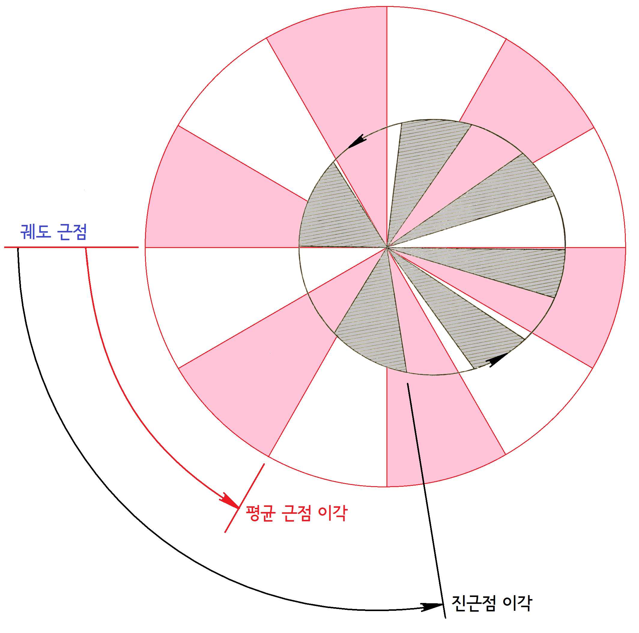
The diagram above shows the areas swept by a planet as it moves along its orbit over equal time intervals. Notice that the gray orbital areas are slightly different from each other, while the pink orbital areas are all equal.
A planet in an elliptical orbit exhibits nonlinear motion according to Kepler’s second law — the law of equal areas. That is, the planet moves faster near perihelion and slower near aphelion.
The mean anomaly represents the angular distance between a body and the perihelion, assuming the body were transferred to a perfect circular orbit while maintaining its orbital speed and period. By simplifying the orbit to a near-circular shape, the angle representing the planet’s position increases linearly with time, making calculations simpler.
Of course, if a planet’s orbital eccentricity were 0 (a perfect circle), the planet would actually move this way. But since most orbits are elliptical, the mean anomaly and eccentricity are used to correct the calculation and determine the planet’s actual motion.
The mean anomaly serves as the most fundamental ingredient for calculating a planet’s position in its orbit. There are several ways to compute it, but since I already have the mean longitude and longitude of perihelion, I’ll use those.
The formula for calculating the mean anomaly from mean longitude () and longitude of perihelion () is:
const meanAnomaly = currentElements.meanLongitude - currentElements.perihelionLongitude;
// 6238.776827293419 degrees
To understand the principle behind this, we need a bit more context on what mean longitude is. The mean longitude used in this calculation represents, on average, how far a planet has progressed in its orbit, measured from the vernal equinox. Mean longitude () can be expressed as:
- : Mean motion (the time for a planet to complete one orbit). This is the total angle of 360°, or radians, divided by the planet’s orbital period.
- : Time elapsed since the reference time . Here, is the J2000 epoch.
- : Longitude of perihelion.
Looking at this formula, when , we get — mean longitude equals longitude of perihelion. This tells us that represents the average angle the planet has traveled from the perihelion.
The final addition of the longitude of perihelion () shifts the reference point of the mean longitude to an angle measured from the vernal equinox.
But what we need is the mean anomaly, which — as its name suggests — uses the perihelion as its reference, not the vernal equinox. So by subtracting the longitude of perihelion from the mean longitude, we shift the reference back to the perihelion.
Calculating the Eccentric Anomaly
Now that we’ve used the mean anomaly to find how far the planet has traveled from perihelion, it’s time to calculate the eccentric anomaly.
The mean anomaly we calculated is like a clock ticking at a constant rate — it simply assumes that since time has passed, the planet must have moved through angle .
But in reality, a planet in an elliptical orbit moves at nonlinear speeds depending on its distance from the central body. So we need to use the mean anomaly and eccentricity to compute the eccentric anomaly, which accounts for the planet’s nonlinear motion — speeding up and slowing down — to find the actual position.
The eccentric anomaly is an angle defined to simplify the actual position of a planet on an elliptical orbit. It represents the central angle when the planet’s position is projected onto an imaginary circular orbit whose radius equals the semi-major axis of the actual elliptical orbit. A diagram makes this more intuitive:
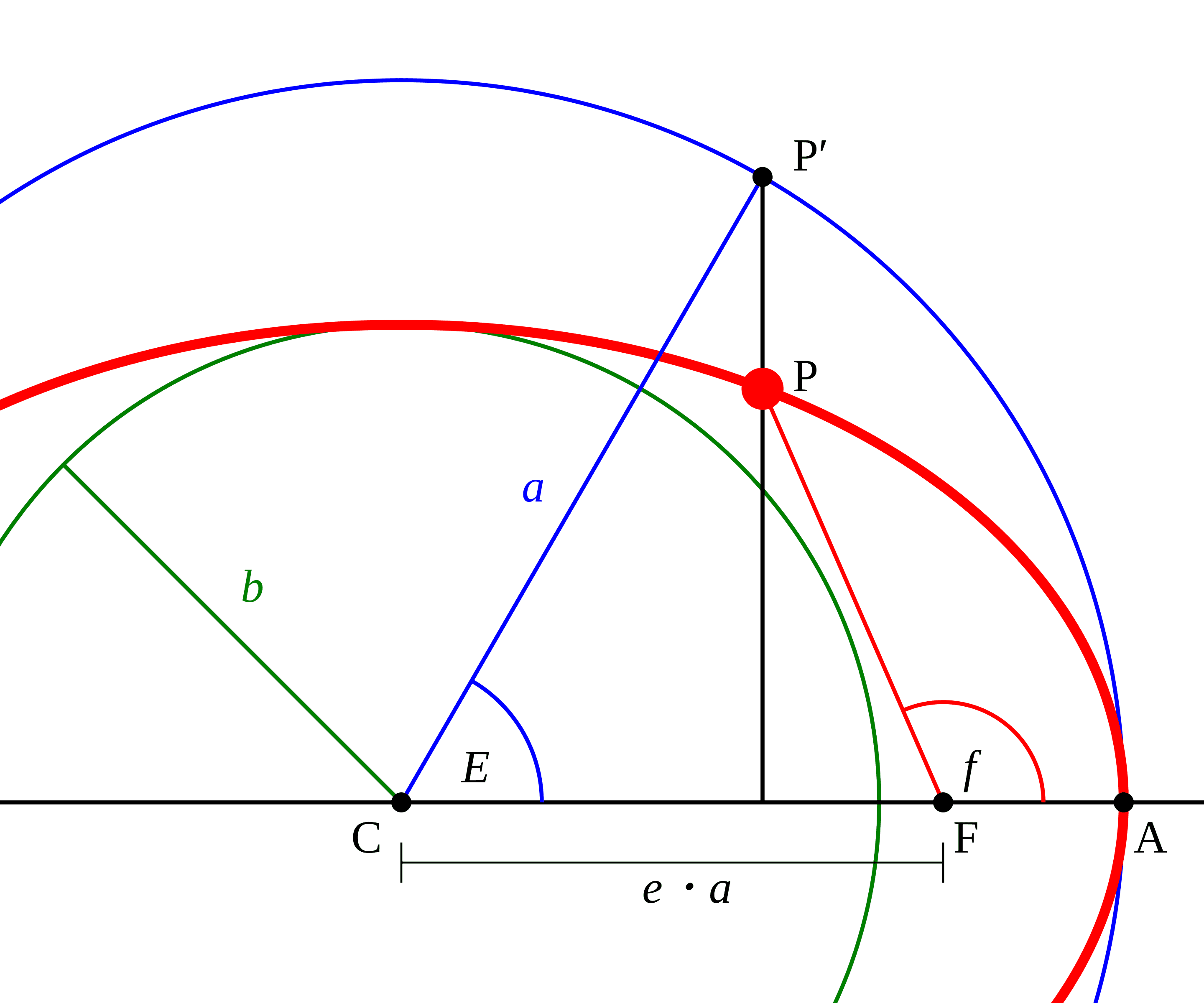
In the diagram, represents the planet’s position on the orbit, and represents the planet’s position projected onto an imaginary circular orbit with radius (the semi-major axis of the actual orbit).
The center of the actual elliptical orbit is , and is one of the ellipse’s foci. The focus represents the gravitational center of the orbit — in the solar system, this would be the Sun. The eccentric anomaly is the angle from the ellipse’s center to the projected position on the imaginary circular orbit.
Like the mean anomaly, the eccentric anomaly represents the planet’s position projected onto an imaginary circular orbit. However, because the eccentricity is factored into the calculation, the eccentric anomaly — unlike the mean anomaly — reflects the geometric characteristics of the elliptical orbit and exhibits a nonlinear rate of increase.
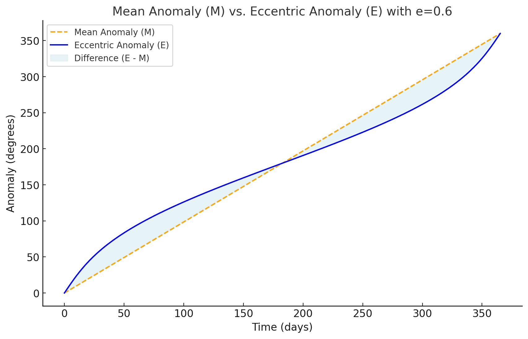 Mean anomaly vs. eccentric anomaly calculated after changing Earth's eccentricity to 0.6 in JPL's orbital elements.
At day 0 (perihelion) the difference is small, but it grows as we approach day 180 (aphelion).
Once we have the eccentric anomaly, we can finally determine the distance from the gravitational center to the actual planet position , as well as the angle — the true anomaly.
Like the mean anomaly, the eccentric anomaly can be derived from multiple definitions. Since I’ve already calculated the mean anomaly, I’ll use the formula derived from it:
This formula calculates the eccentric anomaly using the mean anomaly () and the ellipse’s eccentricity (). The nonlinear characteristics of planetary motion grow stronger with higher eccentricity, which is reflected through the and terms.
Here, adjusts the mean anomaly to account for the nonlinear motion of the ellipse, while acts as a normalization factor indicating whether the planet is closer to perihelion or aphelion.
If , the orbit would be a perfect circle and . But when (an elliptical orbit), near perihelion both and are small so the difference between and is small, while near aphelion both values increase and the difference between and grows.
Unfortunately, the formula for the eccentric anomaly is a nonlinear equation that yields an approximation rather than an exact solution, so we need to reduce the error using the Newton-Raphson method:
Now that we know how to calculate the eccentric anomaly, let’s proceed with the actual computation. Since JavaScript’s trigonometric methods like Math.sin and Math.cos accept radians rather than degrees, we need to convert the mean anomaly to radians:
const convertDegreeToRadian = (degree: number) => degree * (Math.PI / 180);
const meanAnomaly = convertDegreeToRadian(
  currentElements.meanLongitude - currentElements.perihelionLongitude
);
Then we declare a Newton-Raphson helper function and an eccentric anomaly function, and iterate 6 times:
function newtonRaphson<T>(callback: (...args: T[]) => T, initialValue: T, iterations: number) {
  let x = initialValue;
  let x1 = initialValue;

  for (let i = 0; i < iterations; i++) {
    x = x1;
    x1 = callback(x);
  }

  return x1;
}

function getEccentricAnomaly(eccentricity: number, meanAnomaly: number) {
  return (eccentricAnomaly: number) => {
    return eccentricAnomaly + (meanAnomaly + eccentricity * Math.sin(eccentricAnomaly) - eccentricAnomaly) / (1 - eccentricity * Math.cos(eccentricAnomaly));
  };
}

const eccentricAnomaly = newtonRaphson(
  getEccentricAnomaly(currentElements.eccentricity, meanAnomaly),
  meanAnomaly,
  6
);
// 108.9017193604219 radians
Higher eccentricity means larger errors in the getEccentricAnomaly function’s output, requiring more iterations. But since Earth’s orbital eccentricity is about 0.02 — nearly circular — 6 iterations is sufficient.
With the eccentric anomaly calculated, it’s time to use everything we’ve gathered to find the planet’s actual position on the orbital plane.
Finding the Planet’s x, y Coordinates on the Orbital Plane
Now we need to find where the planet is on the orbital plane and express it as and coordinates. The coordinates we’re calculating are relative to the center of the ellipse, but ultimately we’ll use them to determine how far Earth is from the Sun and how many degrees it has traveled from perihelion.
First, the formula for the planet’s coordinate relative to the ellipse’s center:
Since the eccentric anomaly represents the planet’s position projected onto an imaginary circular orbit (because the ellipse’s complex proportions are hard to work with directly), when using the eccentric anomaly to find the planet’s actual position on the elliptical orbit, we need to correct for the difference between the imaginary circular orbit and the actual elliptical orbit.
The term in the formula performs this correction. calculates how far the planet is horizontally from the center on the imaginary circular orbit (based on the eccentric anomaly ). Then subtracting the eccentricity shifts the result by the distance between the ellipse’s center and its focus.
Up to this point, the calculated value is dimensionless — merely a ratio relative to the semi-major axis — so we multiply by the semi-major axis () to set the orbit’s scale.
The formula for the coordinate follows a similar principle:
For the coordinate, first calculates how far the planet is vertically on the imaginary circular orbit, then corrects for the difference between the imaginary circle and the actual ellipse.
The difference here is that we need vertical correction, so we must use the semi-minor axis instead of the semi-major axis. The in the formula is precisely the formula for deriving the semi-minor axis from the semi-major axis and eccentricity.
Now that we understand the general principle, let’s write the code and extract Earth’s coordinates:
const positionX = currentElements.semiMajorAxis * (
    Math.cos(eccentricAnomaly) - currentElements.eccentricity
  );

const positionY = currentElements.semiMajorAxis * (
    Math.sqrt(1 - (currentElements.eccentricity ** 2))
  ) * Math.sin(eccentricAnomaly);
From this, I was able to determine that Earth is located approximately -76,411,956 km along the X-axis and approximately 130,045,428 km along the Y-axis from the center of the ellipse.
Finding the Distance from the Sun and the True Anomaly
We’ve found Earth’s coordinates on the orbital plane, but these coordinates represent the distance from the center of the orbit itself — not from the Sun, which is the gravitational center.
What I actually want to know is Earth’s position relative to the Sun, not the orbital center, so additional calculation is needed. Let’s bring back the diagram from earlier:
Earlier, I calculated the eccentric anomaly shown in the diagram, and used it to find the and coordinates of — the planet’s position on the actual red orbit. But a planet in an elliptical orbit doesn’t orbit the center of the ellipse ; it orbits the gravitational center located at one of the ellipse’s foci.
Since a planet orbiting a gravitational center experiences different gravitational forces depending on its distance, and its orbital speed varies accordingly, what truly matters in orbital calculations is the distance and angle from the gravitational center — not the ellipse’s center.
In other words, I now need to find the distance from (not ) to , and the angle . This angle is called the true anomaly — literally the “true” angle from periapsis.
Let’s first calculate the distance from the Sun to Earth. Since we already have Earth’s and coordinates, the Euclidean distance () from the Sun to Earth can be simply calculated using the Pythagorean theorem:
Here, is the distance from the center of the elliptical orbit to the Sun. Since we calculated Earth’s coordinate relative to the orbital center, we subtract the distance between the orbital center and the Sun to shift the reference to the Sun’s coordinate. Beyond this adjustment, the formula is just the familiar Pythagorean theorem , so I’ll skip the detailed explanation.
const convertKMtoAU = (km: number) => km / 149_597_870;
const distance = Math.sqrt(
  Math.pow(positionX - (currentElements.semiMajorAxis * currentElements.eccentricity), 2) +
  Math.pow(positionY, 2)
);

console.log(convertKMtoAU(distance));
// 1.0168205539250386 AU
Running this calculation tells us that on May 3, 2017, at 10:27 PM, Earth is located approximately 1.02 AU from the Sun.
Now that we have the Sun-Earth distance, let’s calculate the true anomaly to find how many degrees Earth has traveled from perihelion.
While the standard approach derives the true anomaly from the eccentric anomaly, since I already have Earth’s and coordinates, I can use the Math.atan2 function to find the true anomaly directly.
The Math.atan2 function uses the relative positions of y and x to calculate the angle a point forms from a reference point. The result is a radian value between -180° () and 180° ().
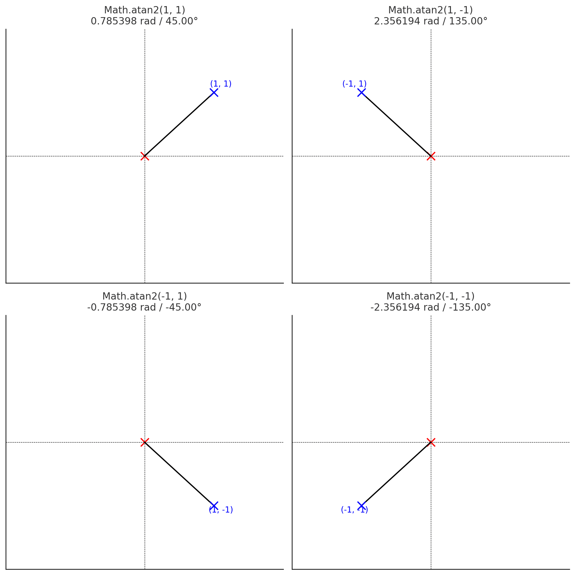 The atan2 function measures angles from the origin relative to the positive x-axis
Note that this function is designed to receive the y coordinate first, as in Math.atan2(y, x). This is because tangent is expressed as , following the form Math.tan(y / x).
The coordinates that Math.atan2 receives aren’t necessarily calculated from the origin — they represent relative coordinates from any arbitrary origin. Since the and coordinates I calculated for Earth are relative to the Sun’s position, plugging them into Math.atan2 directly gives us the angle of Earth’s position relative to the Sun.
const convertRadianToDegree = (radian: number) => radian * (180 / Math.PI);
const trueAnomaly = Math.atan2(
  positionY,
  positionX - (currentElements.semiMajorAxis * currentElements.eccentricity)
);

console.log('True anomaly:', convertRadianToDegree(trueAnomaly));
// 120.4375985828049 degrees
Through this, I was able to determine that as of May 3, 2017, at 10:27 PM, Earth is located approximately 120° from perihelion at a distance of 1.02 AU.
Closing Thoughts
This post only covered finding a planet’s position on the 2D orbital plane. However, once you place the orbit in 3D space by applying the orbital inclination and argument of periapsis, the planet will naturally exhibit three-dimensional motion.
You can check out the simulator I built using these formulas here, and the full source code is available on the Solarsystem project GitHub repository.
That wraps up this post on calculating planetary positions.
관련 포스팅 보러가기
[Simulating Celestial Bodies with JavaScript] Understanding the Keplerian Elements
Programming/Graphics[Implementing Gravity with JavaScript] 2. Coding
Programming/Graphics[Implementing Gravity with JavaScript] 1. What is Gravity?
Programming/GraphicsUsing PayPal's Express Checkout RESTful API
Programming/TutorialWhy Do Type Systems Behave Like Proofs?
Programming