How Do Computers Hear Sound?

Understanding digital audio conversion through sampling, bit rate, and Web Audio API

Jul 10, 2019

In this post, I want to tap into my memories from my former career as a sound engineer and explain some audio theory. But since just explaining theory is boring, I’ll also draw a simple audio waveform using JavaScript’s Web Audio API based on that audio theory.

I want to jump straight into coding, but you need basic knowledge about audio to understand the process of drawing waveforms. So I’ll try to explain the theory in the least boring way possible. Theory is definitely less fun than coding, but these are things you need to know at minimum to draw audio waveforms, so let’s skim through it.

What Is Sound?

First, let’s understand what sound is. If I had to describe sound in one word, it would be “vibration.” Basically, hearing sound happens in this order:

Some object vibrates. Let’s say the vibration frequency is about 440Hz.
The medium around that object transmits the 440Hz vibration (usually air in normal situations).
When the medium transmits the vibration, our eardrum also vibrates at 440Hz.
The cochlea converts that vibration signal into electrical signals and sends them to the auditory nerve.
The brain receives and interprets the signal. 440Hz received!

Here, we use the unit Hertz (Hz) to express how many times the object vibrated in one second in step 1. 10Hz means it vibrated 10 times in one second, and 1kHz means it vibrated 1,000 times in one second.

By the way, 440Hz in the example is the note “A” in do-re-mi-fa-sol-la-ti-do. So when we listen to music, we’re actually feeling vibrations — the vibration of strings for string instruments, the vibration of lips or reeds for wind instruments, and the vibration of vocal cords for singing. Even the most emotional music can be broken down like this in an engineer’s hands.

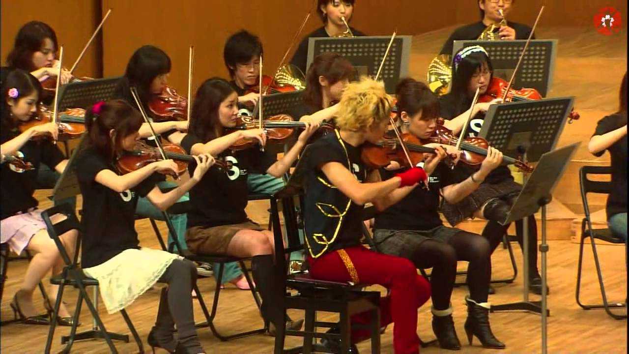The beautiful melodies we hear are just bundles of vibration frequencies when you break them down.

These vibrations occur in nature, so they appear in analog form. Most macroscopic signals occurring in nature are analog — for example, changes in light brightness, wind intensity, or sound volume.

Sound Is an Analog Signal

Analog represents signals or data as continuous physical quantities. This “continuous physical quantities” sounds professional and difficult, but when you break it down, it’s really nothing special. The word we need to focus on here is not “physical quantities” but “continuous.”

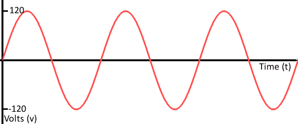The horizontal axis is time, the vertical axis is voltage. Analog signals have continuity that never ends no matter how much you divide them

So what does continuous mean?

The representative example of continuity is numbers. Let’s imagine walking from 1 to 2. How many numbers will we encounter while walking from 1 to 2?

First, at the halfway point between 1 and 2, there’s 1.5. There’s also half of that, 1.25, and half of that, 1.125.

If we keep dividing numbers like this, we eventually realize this is a pointless exercise. Even if we divide down to $10^{-10000}$ units, we can keep dividing that number infinitely. We call this property continuity.

How Computers Hear Sound

But as you know, computers are dumb — they only understand 0 and 1. We call this method digital. So computers that only know 0 and 1 cannot understand continuous analog signals.

Then how can we make a computer hear sound, which is an analog form occurring in nature?

Simple. We convert analog to digital. Once you understand the process of converting the analog signal of sound into something the computer can understand, you’ll know what the information that the Web Audio API gives us means. So let’s learn about the process of converting analog to digital.

To convert analog to digital, we need to go through several steps. The values used in these steps determine the resolution of the digitally converted sound — in other words, the audio quality. The terms that come up here are Sample Rate and Bit Rate.

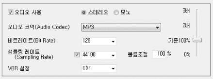Difficult words that make you not know what to adjust when using encoder programs

The terms look difficult, but they’re actually simple. Sound is essentially 2-dimensional vibration frequency data drawn in a space defined by time on the horizontal axis and amplitude on the vertical axis. The sample rate represents the horizontal axis resolution, and the bit rate represents the vertical axis resolution. These values are used in sampling, the first step of converting analog to digital.

Sampling

Sampling is the first step to convert analog signals to digital signals. As explained above, sound as an analog signal is continuous, so computers cannot understand this signal as-is. When we record sound using a microphone, this analog signal is ultimately converted to electrical signals and given to the computer. When sound vibrations reach the device inside the microphone, this device converts them by raising and lowering voltage.

But our dumb computer still can’t understand this electrical signal even after all this.

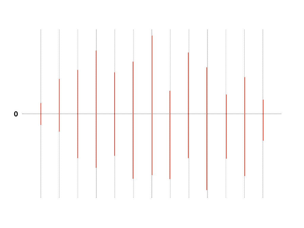
So the computer uses a trick to measure continuous electrical signals by setting specific timings: “I’ll measure voltage at these timings!” Here’s what this trick looks like in a diagram:

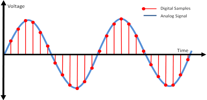
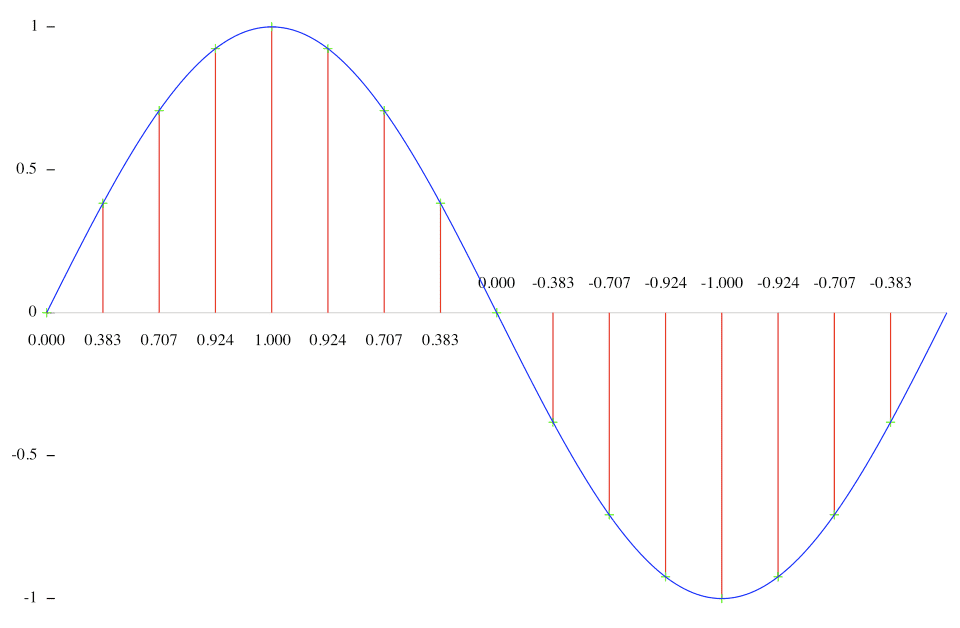
The red dots in the diagram above are the timings when the computer measured voltage. The computer measures electrical signals at specific timings and stores those values. Looking at the red dot positions, this signal would have been measured as something like [10, 20, 30, 27, 19, 8...]. The finer these red dots are — that is, the shorter the intervals at which the computer measures samples — the closer we can get to measuring the original signal.

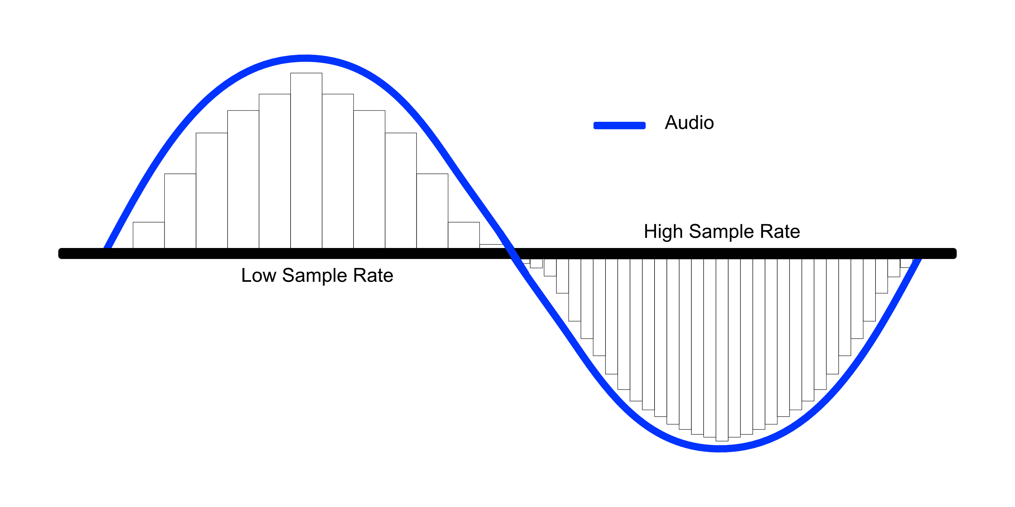The rectangle inside the signal is the shape of the signal as understood by the computer.

The interval at which signals are measured is called the sample rate, and the process of measuring signals itself is called sampling. Naturally, the higher the sample rate, the better the sound resolution — the audio quality. Especially the resolution of high-frequency sounds, meaning high notes, improves noticeably.

Typically, CD audio quality has a sample rate of 44.1kHz, and TV or radio broadcasts have 48kHz. This means about 44,100 or 48,000 samples are measured per second. What criteria determine these sample rates?

Let’s Look at Sample Rate in More Detail

As I just explained, CDs have a sample rate of 44.1kHz. This means the audio on CDs is the result of a computer measuring analog signals 44,100 times per second.

But the range of frequencies humans can hear — the audible frequency range — is only 20Hz ~ 20kHz. So why are sample rates set much higher at 44.1kHz or 48kHz?

Humans can only hear sounds that vibrate up to 20,000 times per second (20kHz), so even if we record sounds vibrating 44,100 times per second (44.1kHz), we can’t hear them anyway, right?

The answer to this question becomes clear when you look at what a sound vibration cycle looks like.

Audio frequencies are basically divided into individual cycles like this. The + part going up is where air compresses, and the - part going down is where air expands again.

As I’ve been explaining, sound is vibration, and what we feel is the air trembling from that vibration. So we need to feel compression > expansion > compression to sense “it vibrated!” In other words, the 20,000 vibrations we can hear means this cycle repeats 20,000 times per second.

You can’t feel “this is vibration” if you only continuously feel either compression or expansion alone.

So to properly measure one cycle of an audio signal, you need to measure both the top peak in the + direction and the bottom peak in the - direction — at minimum 2 measurements are required. So to properly measure 20kHz, the highest sound humans can hear at 20,000 vibrations per second, the computer must measure at least 20,000 * 2 = 40,000 times per second.

This is exactly why CDs have a sample rate of 44.1kHz. This is called the Nyquist Theorem. In short, the Nyquist theorem can be summarized as:

You have an audio frequency you want to measure? If you want to capture the audio signal properly, you need to measure at least twice as fast as that frequency.

So prepare a sample rate at least double the audio frequency you want to measure.

But here another question arises. According to that theory, since the human audible frequency is 20,000Hz, we should be able to record all sounds humans can hear with just 40,000 measurements. So why measure 44,100 or 48,000 times?

Because nature doesn’t only have humans — there are friends like these too:

Hello. I can emit sounds up to 150kHz.

There are actually much higher sounds in nature that we can’t hear. It’s just that we can only hear up to 20kHz. Bats and dolphins make sounds in much higher frequency ranges, don’t they?

So what happens if these sounds enter a container prepared with a 40kHz sample rate? The computer was trying to measure voltage 40,000 times per second to properly measure sounds cycling 20,000 times per second. But what if a much higher frequency sound cycling 30,000 times per second comes in?

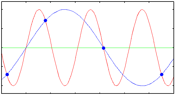
Answer: It starts plotting points in weird places.

Looking at the diagram, the cycle of the incoming signal is shorter than the interval at which the computer plots points — the interval at which it measures voltage. So looking at the points the computer plotted, you can see they’re plotted at awkward places, not at the signal’s peaks. This is the trap that the Nyquist theorem has. And if you connect those awkwardly plotted points (the blue line), you can see it becomes a low frequency. What happens then?

It becomes very audible to our ears. A truly spine-chilling moment! Nothing was audible when recording, but when listening to the recording, there’s a strange sound recorded. So this phenomenon is called “Ghost Frequency.”

Then just crank up the sample rate! Wouldn’t properly recording high sounds solve the problem?

But since this digital audio technology first started being used in the 1970s, hardware capacity couldn’t keep up with arbitrarily raising sample rates.

So the method used to solve this problem was LPF (Low Pass Filter). This filter should be very familiar to those who’ve studied electronics — it literally only passes low frequencies through. If you use an LPF when recording audio to cut off all sounds higher than the human audible frequency and only let sounds in the human audible range pass through, the ghost frequency problem I just mentioned won’t occur.

But analog signals don’t get cut cleanly like cutting radishes.

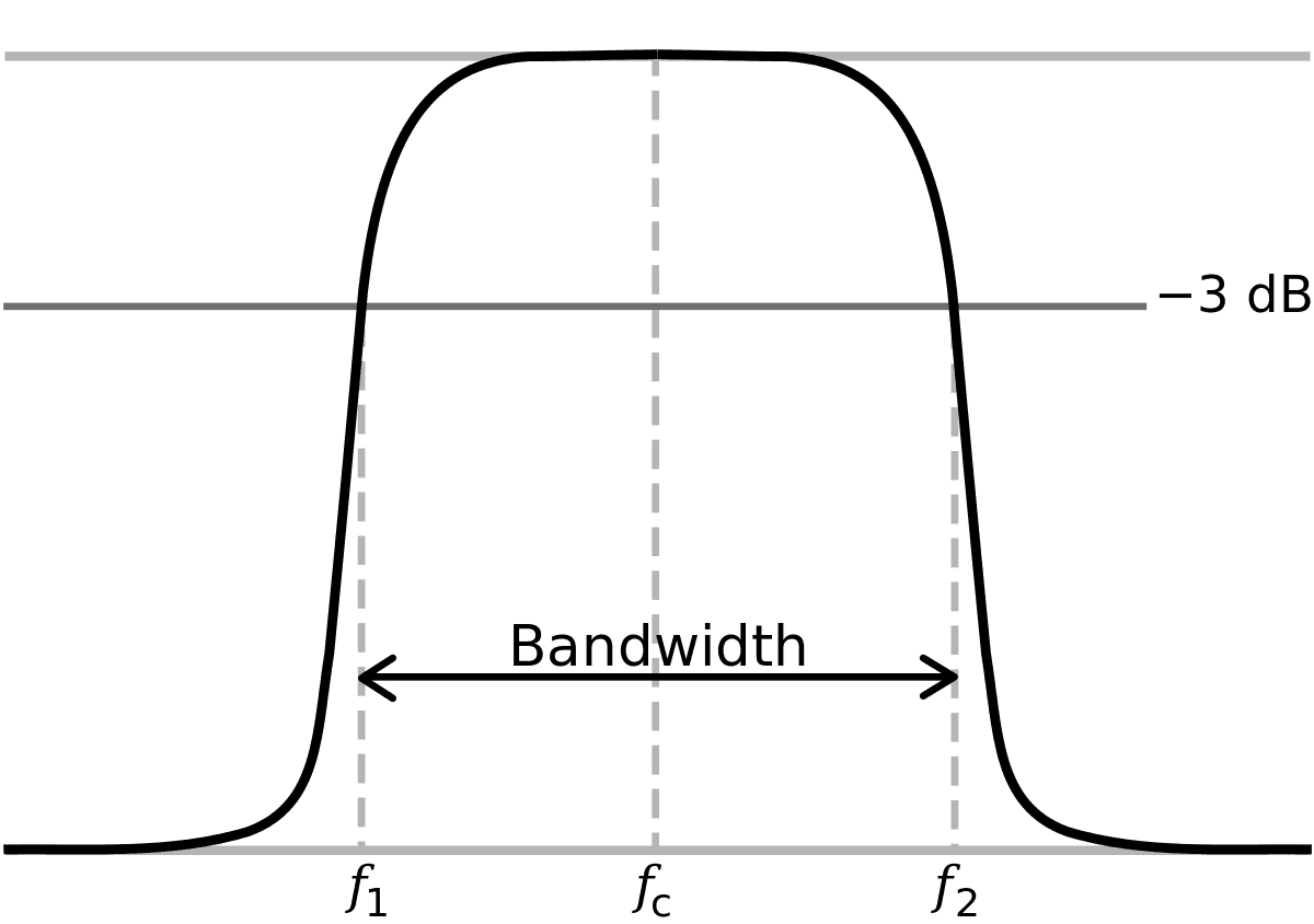
Even with an LPF, the cut portion slopes down diagonally, leaving some less-than-ideal parts. The point where it starts dropping below the allowable range of -3dB shown in the diagram is called the Cut Off. We’re saying we’ll consider the signal cut from there.

You might think, “What if we lower the Cut Off point a bit below 20kHz to make signals disappear around 20kHz?” But apparently they decided it was too wasteful not to utilize the full 20kHz frequency range because of that problem.

So they agreed to set the Cut Off exactly at 20kHz and just accept the remaining portion. With the technology at the time, they reduced and reduced that remaining portion until it was exactly 2,050Hz.

Now if we add the remaining portion and audible frequency, we get 22,050Hz. According to the Nyquist theorem, we need to prepare at least double the sample rate to properly measure this signal, so the standard sample rate for CDs became 44,100Hz = 44.1kHz. There were various other issues that always arise when setting international standards — technical limitations at the time, companies fighting each other, adult matters, etc. — but this was the representative technical reason.

After that, higher sample rates like 48kHz, 96kHz, 192kHz just increased as devices advanced and technical limitations disappeared. “Higher sample rate is better! Let’s pump it up!”

Bit Rate

Bit rate is super simple compared to sampling. Especially since it has “Bit” in the name, which we developers are familiar with, right? If sample rate is the horizontal resolution of sound, bit rate is the vertical resolution.

Like sample rate, bit rate is also commonly explained based on CDs, so I’ll explain based on CDs again.

CD bit rate is 16bit, which literally means it can express values corresponding to 16 bits vertically. When we did sampling earlier as explained above, we measured voltage. The bit rate determines how finely the computer can express these measured voltage values. 16bit means we can use 16-digit binary, and since $2^{16} = 65536$ , we can use a total of 65,537 values from 0 to 65,536.

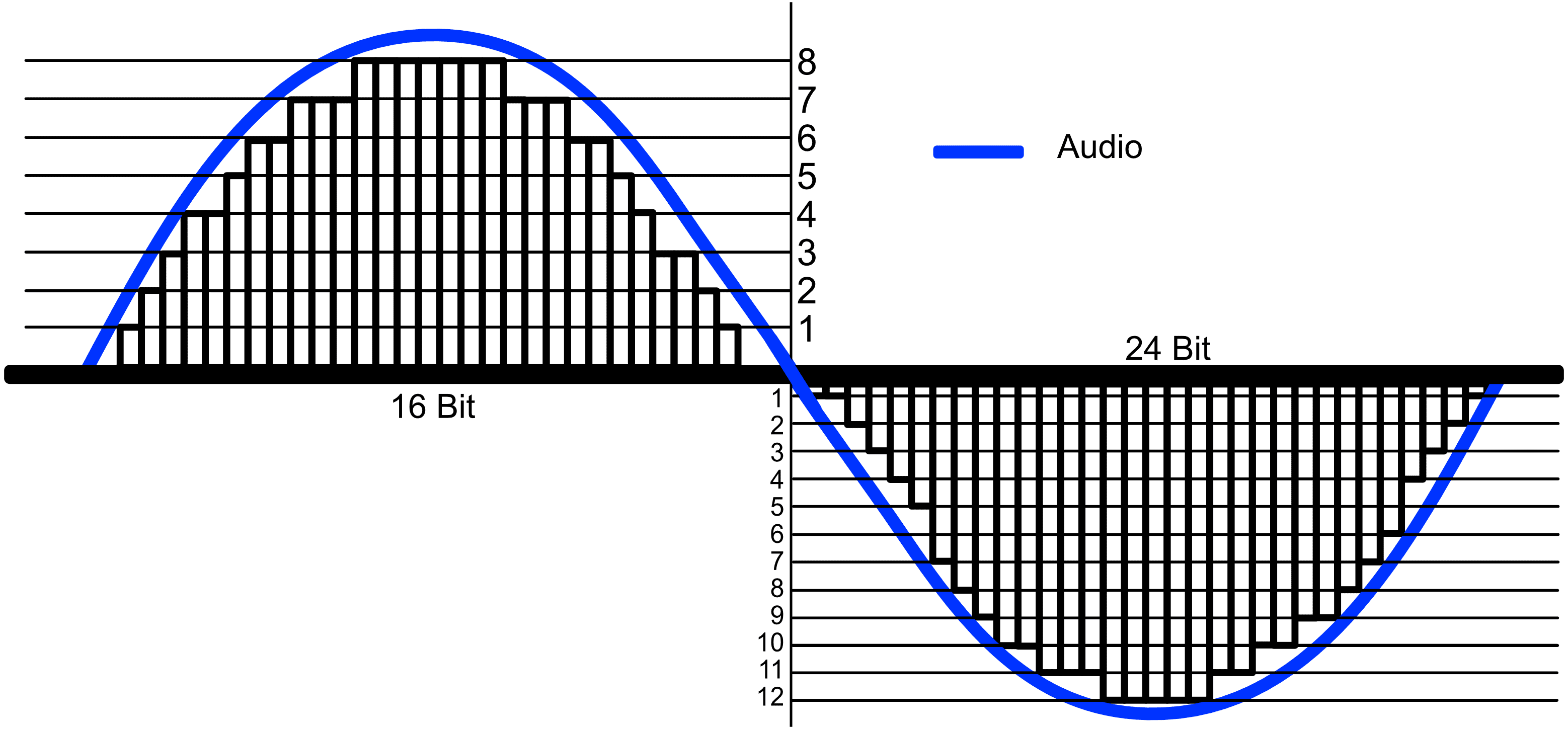You can see that as bit rate increases, the bars inside the analog signal are filled in more meticulously.
Since it's signed counting bits for both + and -, only 50% each is shown in the diagram.

Of course, the voltage values converted from analog sound signals won’t be nice round integers like 123, so we find an approximate value among our available 0-65536 range and convert to it. This process is called quantization. (Yes, it’s the same “quantum” as in quantum mechanics.)

The process of then converting the voltage values changed to 0-65536 into binary that computers can understand is called coding.

Since these are familiar problems for us developers, I’ll just explain this much and move on.

Drawing Waveforms with Web Audio API

Finally, the long audio theory is over. Since my goal is to draw waveforms using digitally converted audio, I only covered the analog to digital conversion process. I won’t cover the reverse process of digital to analog conversion in this post. But that’s also quite interesting, so I highly recommend looking it up separately. I’ll upload an audio file, analyze it with the Web Audio API to extract the needed data, and draw the waveform using svg elements.

For reference, the project was set up super simply using webpack4 and babel7. You can check the detailed code in the GitHub repository.

Setting Up the Basic Structure

Let’s start by writing simple HTML.

<body>
  <input id="audio-uploader" type="file">
  <svg id="waveform" preserveAspectRatio="none">
    <g id="waveform-path-group"></g>
  </svg>
</body>

That’s it for HTML. We just need one input element to upload audio files and one svg element to draw the waveform. Since this is for testing purposes and UI isn’t important, I focused on functionality. (That’s how I’ll spin it.)

Now let’s write an event handler that will execute when a file is uploaded.

// index.js
(function () {
  const inputDOM = document.getElementById('audio-uploader');
  inputDOM.onchange = e => {
    const file = e.currentTarget.files[0];
    if (file) {
      const reader = new FileReader();
      reader.onload = e => console.log(e.target.result);
      reader.readAsArrayBuffer(file);
    }
  }
})();

The FileReader.prototype.readAsArrayBuffer method doesn’t return binary files all at once but returns them in chunk units. It’s commonly used when uploading files to servers and such.

Normally we’d need to write separate logic to handle this ArrayBuffer, but since the Web Audio API we’ll use internally handles ArrayBuffer for us, we don’t need to worry.

Writing the AudioAnalyzer Class

Now it’s time to actually use the Web Audio API. I created a separate singleton class called AudioAnalyzer.

// lib/AudioAnalyzer.js
class AudioAnalyzer {
  constructor () {
    if (!window.AudioContext) {
      const errorMsg = 'Web Audio API not supported';
      alert(errorMsg);
      throw new Error(errorMsg);
    }

    this.audioContext = new (AudioContext || webkitAudioContext)();
    this.audioBuffer = null;
    this.sampleRate = 0;
    this.peaks = [];

    this.waveFormBox = document.getElementById('waveform');
    this.waveFormPathGroup = document.getElementById('waveform-path-group');
  }

  reset () {
    this.audioContext = new (AudioContext || webkitAudioContext)();
    this.audioBuffer = null;
    this.sampleRate = 0;
    this.peaks = [];
  }
}

export default new AudioAnalyzer();

Setting Up the SVG Viewbox

After setting up this basic structure, I’ll declare a method to set the viewbox of the svg element where audio waveforms will be drawn. Since the length of incoming data varies greatly depending on sample rate, we need to dynamically change the viewbox width to match the audio data size so we can draw all signals to fit exactly in the viewbox.

updateViewboxSize () {
  this.waveFormBox.setAttribute('viewBox', `0 -1 ${this.sampleRate} 2`);
}

The viewBox attribute of svg elements means min-x, min-y, width, height from the front. As I mentioned when explaining bit rate, audio signals are signed, so we need to set the viewbox starting at 0, -1 instead of 0, 0. The width is set to the audio’s sample rate so the audio signal fills from start to end of the viewbox, and height is set to 2 since we need to cover -1 ~ 1.

I appropriately added this updateViewboxSize method to the constructor and reset methods so the viewbox size is also initialized when the application initializes.

Checking the Uploaded AudioBuffer

Now we just need to declare a cute setter that decodes audio files uploaded through the input element.

setAudio (audioFile) {
  this.audioContext.decodeAudioData(audioFile).then(buffer => {
    console.log(buffer);
  });
}

The AudioContext.prototype.decodeAudioData method receives an ArrayBuffer and converts it to an AudioBuffer. As I explained above, since the ArrayBuffer returned by the readAsArrayBuffer method doesn’t load all binary data at once but loads in chunk units, decodeAudioData also doesn’t do the conversion synchronously. So when using this method, you need to use callback functions or Promise.

Now let’s change it so that when a file is uploaded, it passes the audio file to AudioAnalyzer so we can see how audio files are actually converted.

// index.js
import AudioAnalyzer from './lib/AudioAnalyzer';

(function () {
  const inputDOM = document.getElementById('audio-uploader');
  inputDOM.onchange = e => {
    const file = e.currentTarget.files[0];
    if (file) {
      // Initialize AudioAnalyzer
      AudioAnalyzer.reset();
      const reader = new FileReader();
      // Pass the file data to AudioAnalyzer
      reader.onload = e => AudioAnalyzer.setAudio(e.target.result);
      reader.readAsArrayBuffer(file);
    }
  }
})();

At this point, I think we don’t need to write anything more in the main function. Now we just play with AudioAnalyzer. To check what data comes out, I uploaded an mp3 file of a song I like.

AudioBuffer {
  length: 12225071,
  duration: 277.2124943310658,
  sampleRate: 44100,
  numberOfChannels: 2
}

Then decodeAudioData executed inside AudioAnalyzer’s setAudio method receives the ArrayBuffer, converts it to AudioBuffer, and returns it. Breaking this down reveals useful information.

sampleRate: Obviously means sample rate — this song’s sample rate is 44,100Hz.
numberOfChannels: Indicates how many channels this audio has — this file is a stereo channel audio file with two channels.
length: Means the number of peaks. Peaks are the voltage values the computer measured during sampling.
duration: Shows this audio file’s playback length in seconds. This song is about 277 seconds long.

Hmm, something to decide here. When audio data with $n$ channels comes in, we need to either express the waveforms of all $n$ channels or merge channels into one and express the waveform. I plan to merge all channels into one even when audio data with $n$ channels comes in.

But explaining channel merging in this post would make things too complicated, so I’ll just proceed using one channel.

Analyzing and Refining Audio Data

Now I’ve obtained the basic audio data, AudioBuffer. With just this data, I can draw audio waveforms. Let’s extract only the needed data from AudioBuffer and assign them to class member variables.

setAudio (audioFile) {
  this.audioContext.decodeAudioData(audioFile).then(buffer => {
    // Assign AudioBuffer object to member variable
    this.audioBuffer = buffer;
    // Assign uploaded audio's sample rate to member variable
    this.sampleRate = buffer.sampleRate;
    // Adjust svg element size according to sample rate
    this.updateViewboxSize();
  });
}

Phew, if we’ve come this far, we’re all ready to draw waveforms. First, let’s extract audio signals one by one from AudioBuffer.

Let’s first look at the array containing audio signals. When I briefly looked at the AudioBuffer data earlier, there was a property called numberOfChannels with value 2 for stereo channels. This channel data can be obtained through the AudioBuffer.getChannelData method.

for (let i = 0; i < this.audioBuffer.numberOfChannels; i++) {
  console.log(this.audioBuffer.getChannelData(i));
}

// Float32Array(12225071) [0, 0, 0, …]
// Float32Array(12225071) [0, 0, 0, …]

Wow, a massive Float32Array appeared. All the values I see now are 0, but that’s because music usually doesn’t start with a BANG! — the elements at later indices have proper values. But we can’t use these values as-is; we need to refine them a bit.

First, let’s think about what those elements in the array actually are. Using the array length 12225071, we can figure out what this friend is. When we looked at this song’s playback duration through AudioBuffer earlier, it was about 277 seconds. Multiplying this song’s sample rate by playback duration gives 12225071. In other words, those elements are the peaks — the voltages the computer measured according to the sample rate.

Each of those peaks is stored as an element in the Float32Array.

Now that we know those elements are peaks, let’s refine these friends a bit. Why refine?

Is rendering all 12,225,071 peaks really efficient visualization…?

A reasonable suspicion. Whether ten million or five million peaks are plotted, we’re going to view it on a small monitor anyway, so expressing every single one doesn’t really have much meaning.

So I’ll compress the peaks appropriately. Instead of collecting all peaks, I’ll create samples of appropriate length and collect only the maximum and minimum values within each sample.

As explained above, according to the Nyquist theorem, we only need one maximum and one minimum to express one cycle, so there’s no problem.

If my application had a waveform zoom feature, I’d need to dynamically select peaks according to how many are needed for rendering when zoom in/out events occur. But this application isn’t that sophisticated, so logic that refines only a fixed number of peaks is sufficient.

const sampleSize = peaks.length / this.sampleRate;
const sampleStep = Math.floor(sampleSize / 10);

// Getting only channel 0 as an example
const peaks = this.audioBuffer.getChannelData(0);
const resultsPeaks = [];

// We'll collect exactly 44,100 peaks, the sample rate length
Array(this.sampleRate).fill().forEach((v, newPeakIndex) => {
  const start = Math.floor(newPeakIndex * sampleSize);
  const end = Math.floor(newPeakIndex + sampleSize);

  let min = peaks[0];
  let max = peaks[0];

  for (let sampleIndex = start; sampleIndex < end; sampleIndex += sampleStep) {
    const v = peaks[sampleIndex];
    if (v > max) {
      max = v;
    }
    else if (v < min) {
      min = v;
    }
  }

  resultPeaks[2 * newPeakIndex] = max;
  resultPeaks[2 * newPeakIndex + 1] = min;
});

It looks complicated, but in one sentence:

Iterate for the sample rate count.

Define a secondary sample section of appropriate length and find max and min within that section.

Insert max at even indices and min at odd indices in the resultPeaks array.

The reason we double the array size with 2 * newPeakIndex when storing values in resultsPeaks is because we need to store up to 2 values, max and min, in each iteration.

This way, I got one appropriately compressed peak array of length 88,200.

Let’s Actually Draw Now!

The drawing method is simpler than you’d think. We just iterate through the peak array we extracted and draw.

SVG’s path element analyzes the string in the d attribute to draw lines. Here, M is Move, a command to move the pointer that draws; and L is Line, a command to draw a line to the specified location.

So we just need to repeat moving the pointer and drawing lines. This is exactly why I stored max values at even indices and min values at odd indices earlier. I intended to use the M command to move the pointer at even indices and the L command to draw lines at odd indices while iterating.

draw () {
  if (this.audioBuffer) {
    const peaks = this.peaks;
    const totalPeaks = peaks.length;

    let d = '';
    for(let peakIndex = 0; peakIndex < totalPeaks; peakIndex++) {
      if (peakNumber % 2 === 0) {
        d += ` M${Math.floor(peakNumber / 2)}, ${peaks.shift()}`;
      }
      else {
        d += ` L${Math.floor(peakNumber / 2)}, ${peaks.shift()}`;
      }
    }

    const path = document.createElementNS('http://www.w3.org/2000/svg', 'path');
    path.setAttributeNS(null, 'd', d);

    this.waveFormPathGroup.appendChild(path);
  }
}

Math.floor(peakNumber / 2) is the $x$ axis, peaks.shift() is the $y$ axis. This code will work roughly like this. Think of the numbers in front as peak indices.

Move pointer to (0, 100)

Draw line to (0, -25)

Move pointer to (1, 300)

Draw line to (1, -450)

Keep repeating

Repeating that process draws bars roughly like this

The audio waveform we’re trying to draw represents digital signals, so it cannot be expressed as continuous analog like the audio signal examples we saw above. So we have to express it by drawing bars like this. It might look like a pretty shabby drawing, but when 88,200 of those lines overlap, it looks pretty convincing.

Even bars become art when drawn well

So, we’ve simply drawn an audio waveform. Now that we’ve done all this… actually there’s a library called WaveSurfer that does this. It has more features too.

I just wanted to try drawing it myself with my own hands.

Music Please, DJ

Just drawing waveforms feels a bit lacking, so let’s make one more method as an interlude. It’s the feature to play this music. Originally my intention when making this method was “let’s at least listen to some music while making this,” but I listened to the same song so many times while making it that I got a bit tired of it.

play (buffer) {
  const sourceBuffer = this.audioContext.createBufferSource();
  sourceBuffer.buffer = buffer;
  sourceBuffer.connect(this.audioContext.destination);
  sourceBuffer.start();
}

The AudioContext.prototype.createBufferSource method creates one of the AudioNodes called AudioBufferSourceNode. When we pass the AudioBuffer we’ve been playing with to this AudioNode, it helps us do real audio control… it’s kind of like a shell.

The Web Audio API provides functionality to modulate sounds by connecting these AudioNodes together, so you can use this to make audio effectors like compressors or reverbs. Next time, I should aim to make an audio effector.

You can check the completed sample source in my GitHub repository, and the live demo here.

That wraps up this post on how computers hear sound.

What Is Sound?
- Sound Is an Analog Signal
How Computers Hear Sound
Drawing Waveforms with Web Audio API
Music Please, DJ