[Deep Learning Series] Understanding Backpropagation

In this post, following the previous post, I want to learn about Backpropagation. As explained earlier, because this algorithm made learning in Multi Layer Networks known to be possible, the Neural Network academic community, which was in a dark age, received attention again.

What is Backpropagation?

Backpropagation is one of the common algorithms for training Artificial Neural Networks today. Directly translating to Korean means 역전파 (reverse propagation). It’s an algorithm that calculates how much difference there is between the target value you want to obtain and the output actually calculated by the model, then propagates that error value back while updating variables each node has.

Fortunately, up to here it’s intuitively understandable, but I was curious about the principles of the following 2 things:

1. How to update variables like weight or bias that each node has?
2. In Multi Layer Networks, variables each node or layer has are all different - how can you know how much to change those values?

Fortunately, these problems can apparently be solved using a rule called Chain Rule. Let’s look step by step.

What is Chain Rule?

Chain Rule, also called the chain rule of differentiation. This isn’t taught in high school but learned in college mathematics, so I, who only learned discrete mathematics in college, had a hard time understanding. Let’s first look at the definition.

When functions $f, g$ exist, if $f$ and $g$ are both differentiable and $F = f(g(x)) = f \circ g$ is a defined composite function, then $F$ is differentiable.

At this time $F'(x) = f'(g(x)) \centerdot g'(x)$.

If we say $t = g(x)$, then $\frac{dy}{dx} = \frac{dt}{dx} \frac{dy}{dt}$ holds.

Looking at the definition, you might wonder what it means. First, composite functions are just functions where other functions are given as arguments to some function. Writing it in code, you can quickly know what feeling it is.

function f(g) {
  return g * 3;
}
function g(x) {
  return x + 1;
}

const x = 3;
let F = f(g(x));
// F = 12

Then what does it mean to be differentiable? If you understand differentiation as something like finding slopes between x and x', you might think “why find slopes in composite functions or whatever?”

But saying find slopes is the same as finding change amounts. Looking at the above code, you can see that when declaring variable F, if you change values given to g, the final F value changes.

F = f(g(4));
// F = 15
F = f(g(2));
// F = 9

In other words, Chain Rule, simply speaking, means you can know how much function g changes when x changes, and how much function f changes due to function g’s change, and if you can know such chain changes, ultimately you can know the contribution of each function f and g contributing to final value F’s change amount.

Just now in the composite function F used as an example above, the variable entering the expression was just one x. Then what happens if there are multiple variables?

In two-variable function $z = f(x, y)$ when $x = h(s,t), y = g(s,t)$

If $f(x,y), g(s,t), h(s,t)$ are all differentiable

can be represented.

This means even if we don’t know how much $s$ or $t$ is, anyway when they change, function $z$’s change amount can be obtained in such expressions.

And $\partial$ is a symbol meaning partial differentiation - it’s a differentiation method that leaves one main variable and completely ignores the rest. So in expressions finding the relationship between $s$ and $z$, you can see $t$ isn’t there at all.

If you understand up to here, now let’s really look at how Backpropagation proceeds.

Forward-propagation

Now let’s directly calculate how Backpropagation is performed.

Before that, we must first proceed with Forward Propagation. After proceeding with calculation using initialized $w$ values and input $x$, we must first find whether desired values come out, and if not, how much they differ.

The model I’ll use for this calculation is as below:

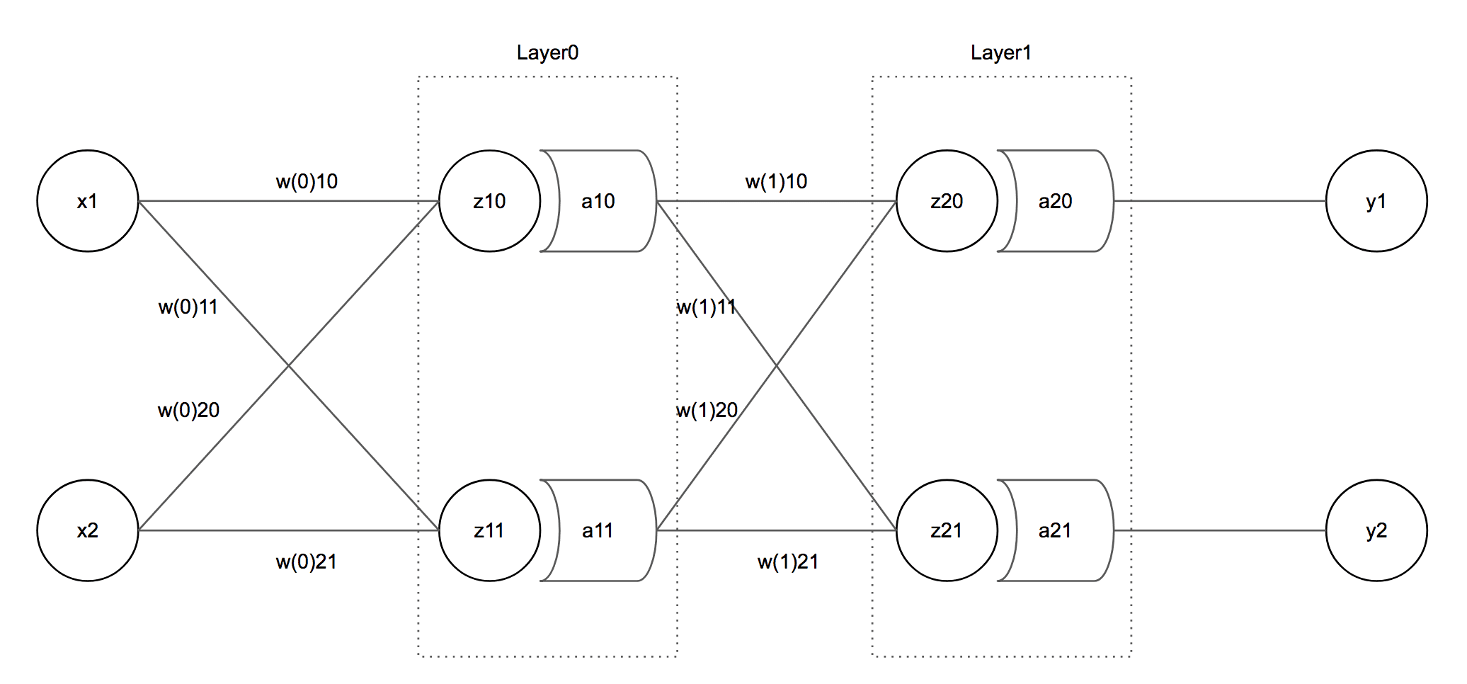
This model is a 2-Layer NN model with 2 inputs, 2 outputs, and 2 Hidden Layers. Now let’s assign values to each variable.

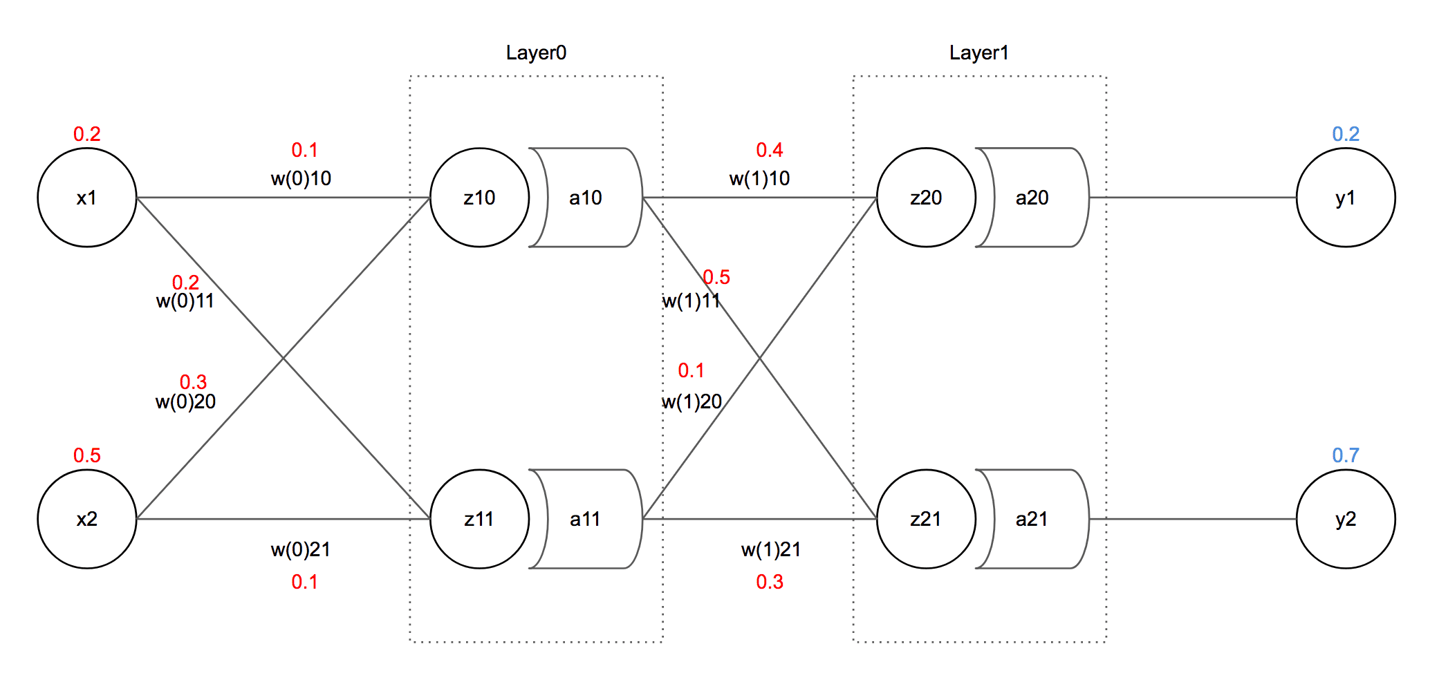
First, $y_1$’s value I want as output is 0.2, $y_2$’s value is 0.7. And as inputs, I put 0.2 in $x_1$ and 0.5 in $x_2$, and just put each $w$ value as feels right.

I want to use Sigmoid function as Activation Function and Mean Squared Error function as Error Function in this calculation.

Let’s first calculate values Layer0 will receive. Usually calculated with matrices.

Unfolding that matrix multiplication becomes as follows and ultimately appears in the form of sums of $wx$.

If we found $z_{10}$ and $z_{11}$ values, now let’s find $a_{10}$ and $a_{11}$ values using Activation Function. The expression for Sigmoid, the Activation Function I’ll use, is as follows:

Since calculating this by hand every time is too cumbersome, I made one function like the following using JavaScript and used it.

function sigmoid(x) {
  return 1 / (1 + Math.exp(-x));
}

Continuing to find values the same way for the next layer, we can find values like the following:

Ultimately, since $y_1$ and $y_2$ are respectively the same as $a_{20}$ and $a_{21}$, we obtained final output values. But $y_1$ and $y_2$ we originally wanted were 0.2 and 0.7, but outputs we obtained are 0.57 and 0.61, with distance.

Now it’s time to find error $E$ using Mean Squared Error function. When calling values we hope to obtain as results $t$ and actual resulting values $y$, error $E$ is as follows:

To explain easily for math dropouts like me, just find how much $y$ values spit out from the final Output Layer differ one by one from labeled $\hat{y}$, then average those values.

Ultimately, training ANN can be seen as approximating this error $E$ value obtained like this to 0. Just backpropagate the $E$ value that came out here.

Since calculating this by hand every time is also annoying, let’s just make one function.

function MSE(targets, values) {
  if (values instanceof Array === false) {
    return false;
  }

  let result = 0;
  targets.forEach((target, i) => {
    result += 0.5 * (target - values[i]) ** 2;
  });

  return result;
}

MSE([0.2, 0.7], [0.57, 0.61]); // 0.072

Now let’s proceed with Backpropagation using error $E$ value found here.

Backpropagation

Looking again at values found through Forward Propagation as a diagram is as follows:

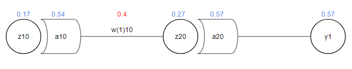
Among these, I want to update the $w^1_{10}$ value currently assigned as 0.4. To do that, I must find how much $w^1_{10}$ affected total error $E$ - that is, contribution. Here the Chain Rule explained above is used.

Unfolding $w^1_{10}$’s contribution to $E$ as an expression is as follows:

Let’s first unfold $\frac{\partial E}{\partial a_{20}}$ in order. Originally $E$ we found was the expression below:

Here, since $a_{20} = y_1, a_{21} = y_2$, I substituted them. But since $\frac{\partial E}{\partial a_{20}}$ is a partial differential expression, just think of $a_{21}$ unrelated to values we’re finding now as 0 and solve.

What this calculation result means is that $a_{20}$, that is $y_1$, contributed 0.37 to total error $E$. Let’s continue calculating like this.

Ultimately we calculated that the value $w^1_{10}$ contributed to $E$ is 0.049. Now putting this value in the learning expression, we can update the $w^1_{10}$ value.

At this time, a value called Learning Rate is needed that decides how much to skip values or how quickly to learn, etc. This is just a constant humans decide, and is usually set lower than 0.1, but I set it as 0.3.

Like this I obtained the new $w^1_{10}$ value 0.3853. Let’s continue updating other $w$ values like this. This time I’ll update the $w^0{10}$ value of Layer0, which is one layer deeper than Layer1.

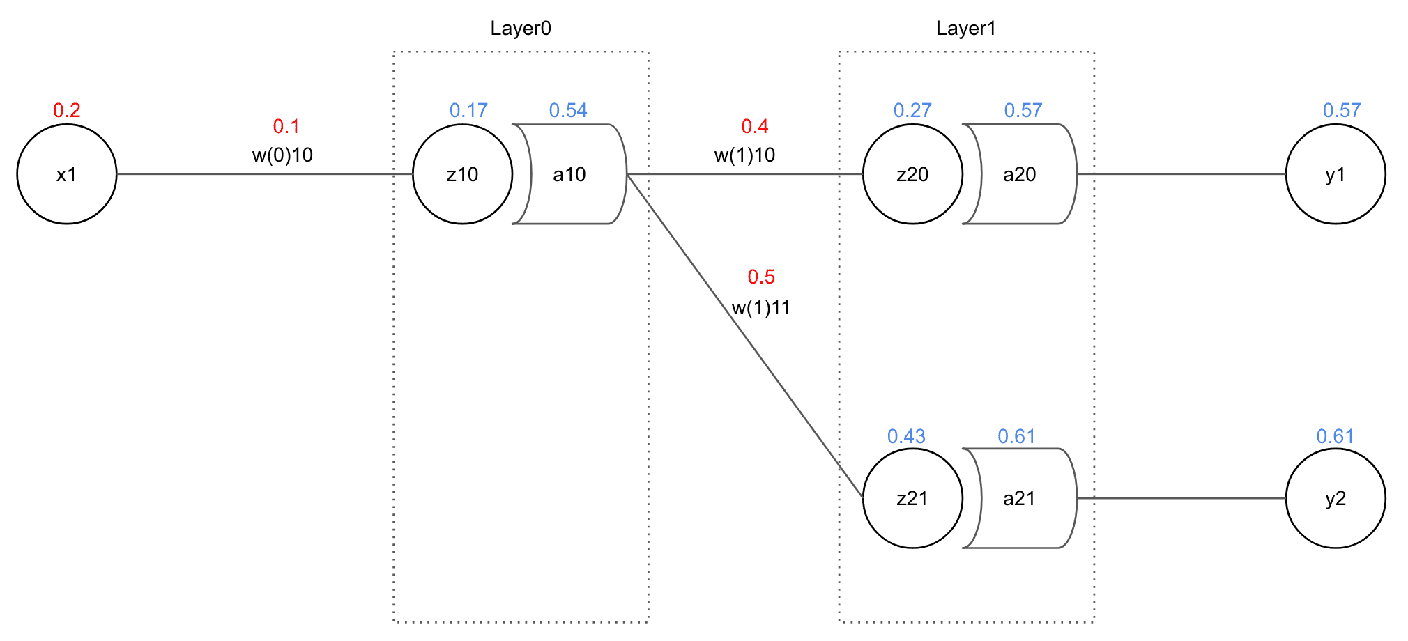
As can be seen, $w^0_{10}$ affects more values than $w^1_{10}$. The degree $w^0_{10}$ contributed to total error $E_t$ can be represented as follows:

Then let’s first find $\frac{\partial E_1}{\partial a_{10}}$.

Similarly, let’s also find $\frac{\partial E_2}{\partial a_{10}}$.

Now that we found all $\frac{\partial E_1}{\partial a_{10}}$ and $\frac{\partial E_2}{\partial a_{10}}$, it’s time to find $\frac{\partial E_t}{\partial w^0_{10}}$.

Thus we found that $w^0_{10}$ contributes 0.0034 to total error $E_t$. Now let’s update the $w^0_{10}$ value using this value. Learning Rate is the same 0.3 as before.

Coding

Since I’m absolutely not a person who can solve this 8 times by hand, I simply wrote the formulas explained above in code using JavaScript.

function sigmoid(x) {
  return 1 / (1 + Math.exp(-x));
}

function MSE(targets, values) {
  if (values instanceof Array === false) {
    return false;
  }

  let result = 0;
  targets.forEach((target, i) => {
    result += 0.5 * (target - values[i]) ** 2;
  });

  return result;
}

// Initialize inputs
const x1 = 0.2;
const x2 = 0.5;

// Initialize target values
const t1 = 0.2;
const t2 = 0.7;

// Initialize Weights
const w0 = [
  [0.1, 0.2],
  [0.3, 0.1],
];
const w1 = [
  [0.4, 0.5],
  [0.1, 0.3],
];
const learningRate = 0.3;
const limit = 1000; // Number of trainings

// Update Weights of second Layer
function updateSecondLayerWeight(targetY, y, prevY, updatedWeight) {
  const v1 = -(targetY - y) + 0;
  const v2 = y * (1 - y);
  const def = v1 * v2 * prevY;
  return updatedWeight - learningRate * def;
}

// Update Weights of first Layer
function updateFirstLayerWeight(t1, t2, y1, y2, w1, w2, a, updatedWeight) {
  const e1 = -(t1 - y1) * y1 * (1 - y1) * w1;
  const e2 = -(t2 - y2) * y2 * (1 - y2) * w2;
  const v1 = a * (1 - a);
  const v2 = a;
  const def = (e1 + e2) * v1 * v2;

  return updatedWeight - learningRate * def;
}

// Start training
let i = 0;
for (i; i < limit; i++) {
  let z10 = x1 * w0[0][0] + x2 * w0[1][0];
  let a10 = sigmoid(z10);
  let z11 = x1 * w0[0][1] + x2 * w0[1][1];
  let a11 = sigmoid(z11);

  let z20 = a10 * w1[0][0] + a11 * w1[1][0];
  let a20 = sigmoid(z20);
  let z21 = a10 * w1[0][1] + a11 * w1[1][1];
  let a21 = sigmoid(z21);

  let e_t = MSE([t1, t2], [a20, a21]);

  console.log(`[${i}] y1 = ${a20}, y2 = ${a21}, E = ${e_t}`);

  // Update with new Weights using calculated contributions
  const newW0 = [
    [
      updateFirstLayerWeight(t1, t2, a20, a21, w1[0][0], w1[0][1], a10, w0[0][0]),
      updateFirstLayerWeight(t1, t2, a20, a21, w1[1][0], w1[1][1], a11, w0[0][1]),
    ],
    [
      updateFirstLayerWeight(t1, t2, a20, a21, w1[0][0], w1[0][1], a10, w0[1][0]),
      updateFirstLayerWeight(t1, t2, a20, a21, w1[1][0], w1[1][1], a11, w0[1][1]),
    ],
  ];
  const newW1 = [
    [updateSecondLayerWeight(t1, a20, a10, w1[0][0]), updateSecondLayerWeight(t2, a21, a10, w1[0][1])],
    [updateSecondLayerWeight(t1, a20, a11, w1[1][0]), updateSecondLayerWeight(t2, a21, a11, w1[1][1])],
  ];

  // Reflect updated Weights
  newW0.forEach((v, i) => {
    v.forEach((vv, ii) => (w0[i][ii] = vv));
  });
  newW1.forEach((v, i) => {
    v.forEach((vv, ii) => (w1[i][ii] = vv));
  });
}

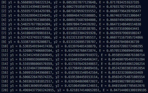
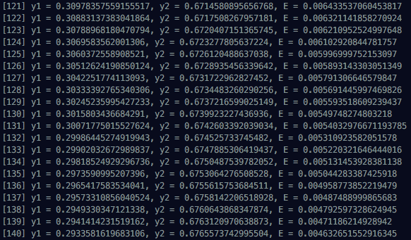
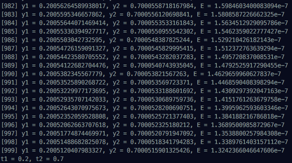
console.log(`t1 = ${t1}, t2 = ${t2}`);

Looking at calculated results, you can see x1 and x2 initially put into Multi Layer Network gradually converging to t1 and t2. Since we can’t see all 1000 run results, I’m attaching first, middle, and last progress situations.

In the next post, I want to create a more structured network. That’s all for this Backpropagation post.