Sharing the Network Nicely: TCP's Congestion Control
How TCP adjusts window sizes to keep the network in harmony

Congestion control is exactly what it sounds like — detecting network congestion and controlling data transmission to resolve it.
The network is such a vast black box that it’s hard to pinpoint exactly where or why transmission is slowing down. But each endpoint can at least detect “things are getting slow.” If you send data and the response from the other party comes late or doesn’t come at all, something is clearly wrong.
When using only the flow control and error control techniques discussed earlier, retransmission inevitably keeps happening.
If just one or two hosts are doing this, it might not be a big deal. But since the network is a shared space used by all sorts of participants, once things start going wrong, everyone starts shouting “I’m retransmitting too!” — making the problem progressively worse. This is called congestion collapse.
So when network congestion is detected, the sender forcibly reduces its data transmission volume by adjusting its window size, in order to avoid this worst-case scenario. This is congestion control.
Congestion Window (CWND)
In my post TCP’s Flow Control and Error Control, I mentioned that the sender’s window size is determined by considering both the receiver’s reported window size and the current network conditions.
When determining its final window size, the sender uses the smaller of two values: the receiver window (RWND) — the window size reported by the receiver — and the congestion window (CWND) — the window size the sender determined based on network conditions.
In other words, the window size that the congestion control techniques below increase and decrease is not the send window itself, but the sender’s “congestion window size.”
Note that since both RWND and CWND have “window” in their names, you might think they’re the same as the window used in sliding window. But they’re just numbers representing the receiver’s window size and the congestion window size, respectively.
So while the congestion window size can be flexibly adjusted based on network congestion during communication, how is it initialized before communication even starts?
Initializing the Congestion Window Size
During communication, information like lost ACKs or timeouts can be used to infer network congestion. But before communication begins, none of that information exists, making it tricky to set the congestion window size. This is where MSS (Maximum Segment Size) comes in.
MSS represents the maximum amount of data that can be sent in a single segment, and can be roughly calculated as:
MSS = MTU - (IP header length + IP option length) - (TCP header length + TCP option length)
MTU (Maximum Transmission Unit) represents the maximum unit that can be sent in a single transmission.
In other words, MSS tells you how much space is left for actual data after stripping away all the non-data parts like IP and TCP headers from the maximum transmission unit.
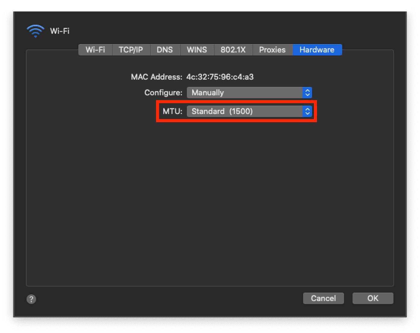 If you dig around in system preferences, you can find a setting to change the default MTU
On macOS, the default MTU is set to the Ethernet standard of 1500 bytes. If the TCP and IP headers are each 20 bytes, then MSS is 1500 - 40 = 1460 bytes.
The sender initializes the congestion window size to 1 MSS when first starting communication. From there, it increases or decreases the congestion window size based on network congestion as communication proceeds.
Congestion Avoidance Methods
TCP, the grandpa protocol, has accumulated a diverse set of congestion control policies over the past 50 years.
Each policy has evolved by improving how to identify congestion and how to increase or decrease the congestion window size. But the most fundamental congestion control approach combines two avoidance methods — AIMD and Slow Start — as the situation demands.
So in this post, I’ll first explain AIMD and Slow Start, then discuss the representative congestion control policies Tahoe and Reno.
AIMD
AIMD (Additive Increase / Multiplicative Decrease) means exactly what it says. When the network seems fine and you want to speed up transmission, you increase the congestion window size by 1. But when congestion is detected — data loss, missing responses — you cut the congestion window size in half.
Increase: ws + 1. Decrease: ws * 0.5. Literally additive increase, multiplicative decrease. Because of this characteristic — linear growth and sharp halving — graphing the congestion window size of a connection using AIMD produces a sawtooth pattern.
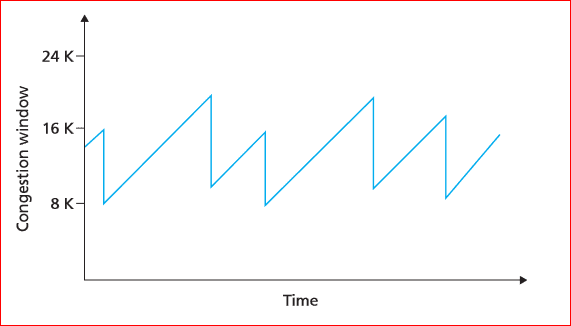 Gradual increase, sharp decrease
This approach is remarkably simple, yet surprisingly fair. Imagine several hosts are already occupying the network when a latecomer joins.
Naturally, the latecomer starts with a smaller congestion window and is at a disadvantage. But when congestion hits, the host with the larger window is more likely to lose data from trying to push too much through. That host then reduces its window size to resolve the congestion, freeing up bandwidth for the latecomers to grow their windows.
Over time, regardless of when each host joined the network, all hosts’ window sizes converge to an equilibrium.
However, AIMD’s weakness is that even when bandwidth is plentiful, it increases the window size too slowly. It takes time to reach full network utilization.
Window Sizes Really Converge?
AIMD is simple enough that you can simulate the network behavior with a basic example. Doing so lets you actually see what “window sizes converging to equilibrium” means.
I was going to include the code in this post, but trying to simulate something close to real network conditions made it longer than expected, so I’ll just share the results. Here’s my experimental setup:
- Maximum network congestion is
50, determined by the sum of all hosts’ congestion window sizes.- A new host is added to the network every
300ms.- Each host calculates current network congestion every
100-200msand adjusts its window size.- Each host performs 300 window size adjustments before leaving the network.
A small caveat: I used setInterval for concurrency, but since setInterval callbacks go through the event loop and execute on the call stack, true parallelism isn’t guaranteed like in a real network. But this doesn’t affect the test’s purpose — verifying that latecomers can achieve adequate congestion window sizes.
For more on this concept, check out my post A Low-Level Look at the Node.js Event Loop.
Here’s the time-series visualization of the test data. First, let’s look at each host’s congestion window size changes:
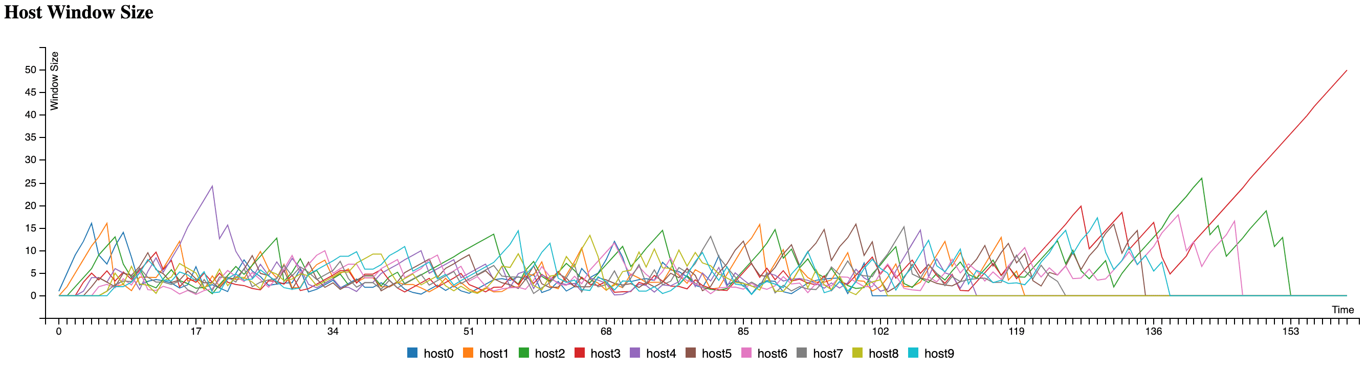
The graph shows that early arrivals and latecomers don’t have dramatically different congestion window sizes. The lone spike at the end is from the last host having the network all to itself after everyone else left.
This visualization confirms that each host’s congestion window size converges to roughly the same range. What about the total window size of all hosts in the network?

The total congestion window sizes across all hosts clearly stay below the congestion threshold of 50 I set, with hosts jockeying back and forth to adjust their window sizes.
Excluding the early and late phases when hosts are joining and leaving, the middle portion shows that individual congestion window sizes don’t vary significantly.
Running this simulation and seeing the data made the abstract concept of “window sizes converging to equilibrium” much more tangible.
If you’d like to run the code yourself and observe the entire process, you can clone it from my GitHub repository.
Slow Start
As mentioned, AIMD increases window size linearly, so it takes a while to reach proper speed.
These days, with generous network bandwidth and excellent infrastructure, congestion occurs far less frequently than before. This has made AIMD’s drawback — taking too long to reach full speed even when no congestion exists — increasingly prominent.
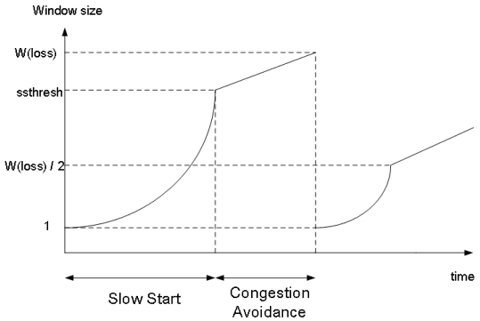
Slow Start shares the same basic principle as AIMD, but increases the window size exponentially. When congestion is detected, it drops the window size to 1.
This approach increases window size each time an ACK arrives, so it may start slowly, but the window grows progressively faster over time.
Since the only difference from AIMD is how the window size increases and decreases, adjusting the window-sizing logic in the earlier example produces a Slow Start chart:
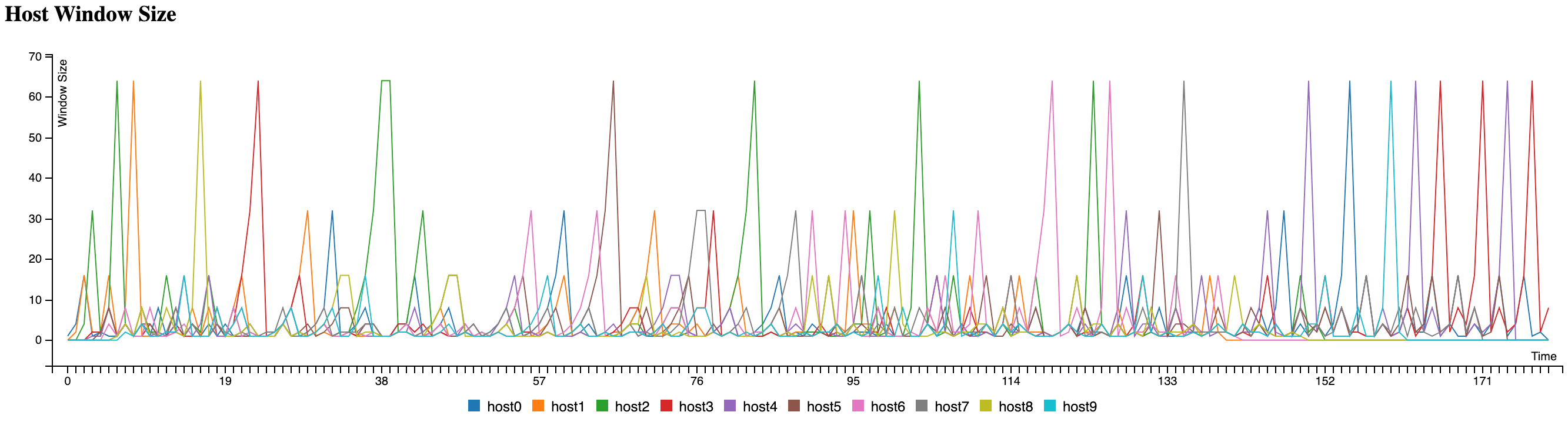
You’ll notice cases where hosts’ congestion windows exceed the maximum congestion threshold of 50 I set. This is an artifact of how JavaScript processes setInterval callbacks and wouldn’t happen in a real network. (The congestion calculation is also far more complex in reality.)
The biggest difference between the AIMD and Slow Start graphs is the time to reach peak network congestion.
AIMD grows window size linearly, so it can’t claim much bandwidth when new hosts join. Slow Start grows slowly at first but then ramps up exponentially when there’s still headroom, ultimately growing the window size faster than AIMD.
Modern TCP policies like Tahoe and Reno blend AIMD and Slow Start, differing primarily in how they respond when congestion occurs.
Congestion Control Policies
TCP has a dizzying array of congestion control policies — Tahoe, Reno, New Reno, CUBIC, and even the recent Elastic-TCP, to name just a few.
These policies all share the premise that when congestion occurs, you reduce (or stop increasing) the window size to avoid it. Newer methods detect congestion more intelligently and utilize network bandwidth more quickly and safely.
Covering all of them here would be impractical, so I’ll focus on the most representative and well-known policies — Tahoe and Reno — to explain the fundamentals of congestion control.
Both Tahoe and Reno start with Slow Start, then switch to AIMD when the network feels congested.
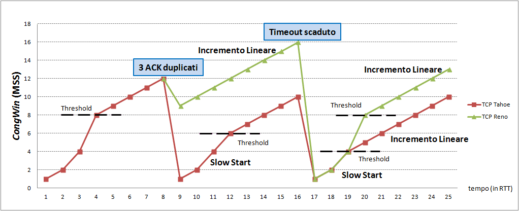 Red represents Tahoe, green represents Reno's window size
The Y-axis shows the congestion window and the X-axis shows time. Before diving into Tahoe and Reno, let me quickly cover a few terms to help you understand what this graph is showing.
Let’s look at the “3 ACK Duplicated” and “Timeout” labels where the graph bends, and the “Threshold” where the growth rate changes. (The spelling in the diagram looks off because it’s Italian, not English — don’t worry about it.)
3 ACK Duplicated, Timeout
Both methods reduce the window size when two scenarios occur: 3 ACK Duplicated and Timeout. These are the fundamental situations that congestion control policies use to detect congestion.
Timeout means the sender’s data was lost or the receiver’s ACK was lost due to various factors.
3 ACK Duplicated — receiving the same acknowledgment number three or more times — is also abnormal. Since the receiver only sends ACKs for data it successfully processed, receiving the same acknowledgment number three times suggests the receiver couldn’t properly process data after a certain sequence number.
However, since TCP uses packet-based transmission where arrival order isn’t guaranteed, one or two duplicate acknowledgment numbers don’t immediately indicate congestion.
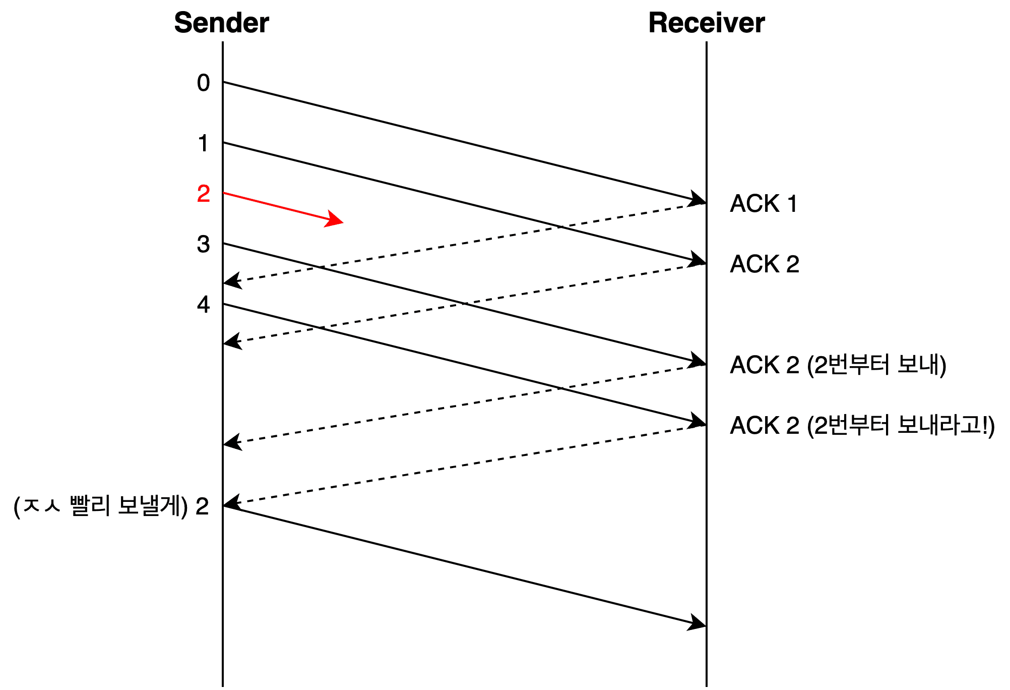
TCP uses cumulative acknowledgment — it sends the acknowledgment number for the last correctly received data in sequence. So if the sender keeps receiving the same acknowledgment number, it knows that data up to that point was transmitted successfully, but something went wrong after that.
When 3 duplicate ACKs trigger immediate retransmission of the corresponding data, the receiver then uses its error control method (Go Back N or Selective Repeat) to tell the sender which packets to send next.
In this situation, the sender can retransmit the packet immediately without waiting for its timeout — a technique called Fast Retransmit.
Without Fast Retransmit, the sender would have to wait until its timeout expires before responding, wasting time before retransmitting the errored data.
Slow Start Threshold (ssthresh)
Looking at the Tahoe vs. Reno graph, you’ll notice the word “Threshold” appearing frequently. This refers to the Slow Start Threshold (ssthresh), meaning “I’ll only use Slow Start up to this point.”
The reason for this threshold is that exponentially increasing window size with Slow Start eventually leads to uncontrollable growth. When congestion seems imminent, it’s much safer to increase cautiously and incrementally rather than aggressively.
Think of it simply: if the current window size is 10 and the remaining network capacity is 15, Slow Start would blow past 20, but additive increase gives you about 5 more rounds of safe growth.
So a threshold is set, and once exceeded, AIMD’s linear increase is used instead. That’s why it’s called the Slow Start Threshold.
The sender initializes ssthresh to half its congestion window — 0.5 MSS — before communication begins, then responds differently depending on which congestion control method is being used.
TCP Tahoe
TCP Tahoe is an early congestion control policy using Slow Start, and the first to introduce the Fast Retransmit technique. Policies developed after Tahoe use Fast Retransmit as a baseline, adding refinements for efficiency.
Fun fact: TCP Tahoe is named after Lake Tahoe in Nevada. So it’s pronounced “Tah-ho.” (Not “Tah-ho-ay”!)
 I'm not sure why they named it after this lake, but it is beautiful
Tahoe starts with Slow Start, exponentially increasing its window size until hitting the Slow Start Threshold, then switches to AIMD’s additive increase for linear growth.
When 3 ACK Duplicated or Timeout occurs, it determines that congestion has happened and modifies both the Slow Start Threshold and its window size. Let’s look at Tahoe’s congestion window graph for a clearer picture:
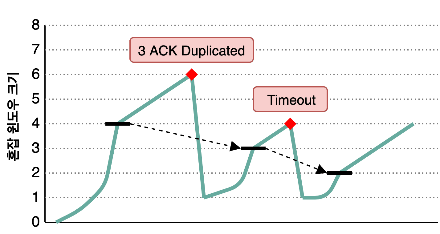
The teal line shows the sender’s congestion window size, and the bold black line shows ssthresh. In this scenario, the initial congestion window is 8, so ssthresh is set to 8 * 0.5 = 4.
The sender exponentially increases its window size using Slow Start until hitting ssthresh, then switches to linear increase. What happens when congestion (3 ACK Duplicated or Timeout) occurs?
At the first congestion event, the congestion window is 6. The sender sets ssthresh to half of that — 3 — and resets its congestion window to 1. Then it starts Slow Start again, switching to additive increase upon reaching the threshold. Rinse and repeat.
In essence, it remembers where it got hit last time and starts being cautious as it approaches that point. A reasonable approach.
But there’s no silver bullet. Tahoe’s weakness is that the initial Slow Start phase takes too long to grow the window. While exponential growth is faster than additive growth overall, resetting the window to 1 after every congestion event is arguably wasteful.
This led to TCP Reno, which uses the Fast Recovery approach.
TCP Reno
TCP Reno was developed after Tahoe. Like Tahoe, it starts with Slow Start and switches to additive increase after the threshold.
But Reno has a clear difference: it distinguishes between 3 ACK Duplicated and Timeout. When 3 duplicate ACKs occur, Reno doesn’t drop the window to 1 — it halves it (like AIMD) and sets ssthresh to the reduced window value.
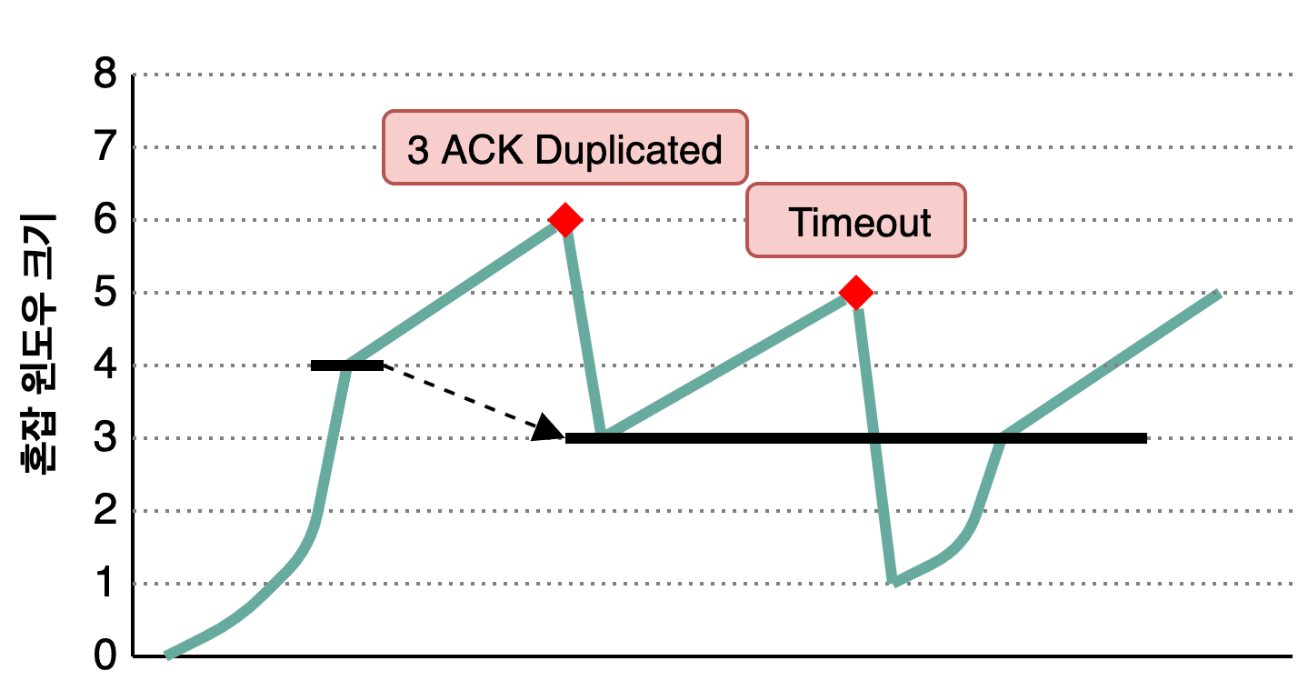
The graph above uses the same notation — teal for the congestion window, bold black for ssthresh.
Unlike Tahoe, when 3 duplicate ACKs occur, Reno halves the congestion window and proceeds with additive increase from there. Since this avoids resetting to 1 and starting from scratch like Tahoe, it reaches the previous window size much faster — hence the name Fast Recovery.
The ssthresh is set equal to the reduced window size. In the graph, when congestion occurs, the window drops from 6 to 3, and ssthresh is also set to 3.
However, if data is lost due to a timeout, Reno drops the window to 1 just like Tahoe and proceeds with Slow Start — without changing ssthresh.
In other words, it differentiates between duplicate ACKs and timeouts, responding differently to each. By assuming duplicate ACKs indicate less severe congestion than timeouts and not dropping the window to 1, Reno effectively weighs the severity of congestion situations.
Wrapping Up
This post covered TCP’s congestion control policies. Honestly, Tahoe and Reno are somewhat dated — they’re not widely used in modern networks.
Being designed for the network conditions of their era, they don’t quite fit today’s high-bandwidth networks.
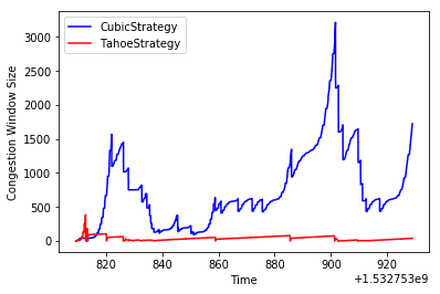 The efficiency gap between Tahoe and CUBIC at high bandwidth is staggering
Compared to when Tahoe and Reno were developed, today’s network bandwidth is probably at least 1,000 times more generous.
This means the probability of problems when a sender aggressively grows its congestion window is much lower than before. So modern congestion control policies focus on how to grow the congestion window faster and how to detect congestion more intelligently.
 TCP CUBIC, which leverages cubic function properties, barely increases window size while avoiding congestion, then explosively ramps up once congestion clears
The reason I introduced the older Tahoe and Reno is that as early TCP congestion control methods, their principles are straightforward, and later methods don’t fundamentally deviate from the same mechanisms.
This post aimed to understand how the congestion control mechanism works as a whole, not to catalog every policy. So I intentionally left out other congestion control approaches.
If you’re curious about modern congestion control policies, check out these links:
That concludes this post on sharing the network nicely with TCP’s congestion control.
관련 포스팅 보러가기
TCP's Flow Control and Error Control
Programming/NetworkHow TCP Creates and Terminates Connections: The Handshake
Programming/NetworkWhat Information Is Stored in TCP's Header?
Programming/NetworkWhy Did HTTP/3 Choose UDP?
Programming/NetworkThe Path from My Home to Google
Programming/Network