Diving Deep into Hash Tables with JavaScript

In this post, I want to cover the hash table — one of the most commonly used data structures. Let’s start by understanding what a hash table is and why we use it.

What is a Hash Table?

A hash table is a data structure that takes an input value, passes it through a hash function, and stores it at the index returned by that function. It’s usually implemented using arrays. Before explaining what a hash function is or what “hash” even means, let’s first understand where the concept of hash tables originated.

Direct Address Table

The idea behind hash tables evolved from a data structure called the Direct Address Table. A direct address table is a data mapping approach that uses the input value directly as the key. Code makes this easier to understand:

class DirectAddressTable {
  constructor () {
    this.table = [];
  }

  setValue (value = -1) {
    this.table[value] = value;
  }

  getValue (value = -1) {
    return this.table[value];
  }

  getTable () {
    return this.table;
  }
}

const myTable = new DirectAddressTable();
myTable.setValue(3);
myTable.setValue(10);
myTable.setValue(90);

console.log(myTable.getTable());

If you’re reading this post on a desktop, copy and paste this code into your browser console or Node.js and run it. You’ll see our beautiful table printed to the console:

[ <3 empty items>, 3, <6 empty items>, 10, <79 empty items>, 90 ]

When we put 3 into the table, it becomes the element at index 3. When we put 90, it becomes the element at index 90. Super simple. With a direct address table, knowing the input value means knowing the index where it’s stored, so we can access the stored data directly.

myTable.getValue(3); // 3

Since the value we’re looking for equals the table’s index, we can access the storage location directly without searching through the table — giving us $O(1)$ time complexity. Similarly, inserting, updating, or deleting values in the table can all be done in one shot if we know where the value is, also achieving $O(1)$ time complexity.

The reasons why algorithms for searching, inserting, updating, and deleting values in simple data structures like this tend to be time-consuming are usually similar:

1. I don’t know where my target value is. Let’s search efficiently. (e.g., binary tree search)
2. Inserting or deleting this value affects other values. (e.g., linked list)

The direct address table is very convenient because we know exactly where our target value is, allowing direct access for subsequent operations.

But direct address tables have an obvious downside: poor space efficiency. Looking at the state of myTable we just created makes this immediately clear. We inserted 3, 10, and 90 — values with quite large gaps between them.

As a result, our myTable stores data in this sparse structure:

Array(91) [
 0, 0, 0, 3, 0, 0, 0, 0, 0, 0, 10, 0, 0, 0, 0, 0, 0, 0, 0, 0,
 0, 0, 0, 0, 0, 0, 0, 0, 0, 0, 0, 0, 0, 0, 0, 0, 0, 0, 0, 0,
 0, 0, 0, 0, 0, 0, 0, 0, 0, 0, 0, 0, 0, 0, 0, 0, 0, 0, 0, 0,
 0, 0, 0, 0, 0, 0, 0, 0, 0, 0, 0, 0, 0, 0, 0, 0, 0, 0, 0, 0,
 0, 0, 0, 0, 0, 0, 0, 0, 0, 0, 90]

As you can see above, the spaces filled with 0 (except for the stored data) have memory allocated but hold no values. In other words, wasted space. When using a direct address table, if the number of values is smaller than the range of data values you want to store, space efficiency suffers.

This situation is described as having a low load factor. The load factor is calculated as number of values / table size. The current load factor of my table is 3/91 = 0.03296..., about 3% — not a high load factor.

If even one large value like 1000 enters the table, the table size becomes 1001 and the load factor drops to 0.003996..., about 0.4%. In other words, direct address tables work best when storing consecutive values like 1, 2, 3 or data where values don’t have large range differences.

Compensating for Direct Address Table’s Weakness with Hash Functions!

So direct address tables are convenient for accessing values but have poor space efficiency. Hash tables were designed to compensate for this weakness.

Instead of using the value directly as the table index like a direct address table, a hash table passes the value through something called a hash function first. A hash function maps arbitrary-length data to fixed-length data. The output of this function is called a hash.

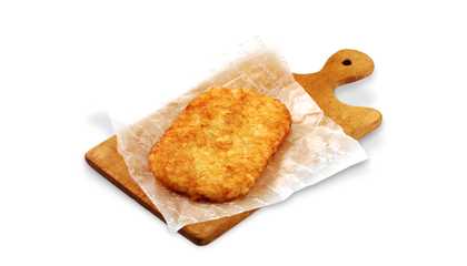The word "hash" originally means something like "chopped up food" — think of a hash brown.
A hash function works similarly: whatever value comes in, it gets mashed into a fixed-length output.

Let me create a simple hash function to help with understanding:

function hashFunction (key) {
  return key % 10;
}

console.log(hashFunction(102948)); // 8
console.log(hashFunction(191919191)); // 1
console.log(hashFunction(13)); // 3
console.log(hashFunction(997)); // 7

That’s it. Sure, it’s a crude hash function, but it does perform its core job of hashing just fine.

My crude hash function simply divides the input by 10 and returns the remainder. Since only the ones digit is returned regardless of input, the output is guaranteed to be between 0-9.

One characteristic of hash functions is that looking at the hash alone makes it hard to guess what the input was. You can’t determine the original number just by looking at the ones digit. This is why hash functions are widely used in cryptography.

But what’s important for us isn’t cryptography — it’s this:

No matter what value goes into the hash function, it will always return a value between 0-9!

The weakness of direct address tables was that even if just one value like 10000 came in, you’d need to create a table of size 10000 to store it at index 10000, wasting 9999 spaces.

But with my hash function, 100 returns 0, 10001 returns 1, and even 8982174981274 returns 4.

This means we can set a fixed table size and store data only within that space. Let me write a simple hash table using this property of hash functions. I’ll set the hash table size to 5 and write a hash function that ensures any value can be stored in this table.

const myTableSize = 5;
const myHashTable = new Array(myTableSize);

function hashFunction (key) {
  // Divide the input by table size and return the remainder
  return key % myTableSize;
}

myHashTable[hashFunction(1991)] = 1991;
myHashTable[hashFunction(1234)] = 1234;
myHashTable[hashFunction(5678)] = 5678;

console.log(myHashTable); // [empty, 1991, empty, 5678, 1234]

The input values 1991, 1234, and 5678 are much larger than my hash table size of 5, but since the hash function only returns values between 0-4, the values get stored neatly in my small, cute hash table.

My hash table... so tiny and cute

And just like that, we’ve eliminated the endlessly wasted space that was the direct address table’s weakness!

Hash Collision

It would be nice if this were a happy ending, but hash tables have their own weakness: hash collisions. Before explaining what a collision is, let’s use my hash function to create one and see for ourselves:

hashFunction(1991) // 1
hashFunction(6) // 1

When different values put into a hash function produce the same output — that’s a collision.

If you think about it logically, direct address tables grew dynamically, but hash tables allocate fixed space upfront and keep cramming values into it.

So if you set the table size to 100 and try to insert 200 pieces of data, only 100 will be stored and 100 will be left over — what happens to them?

Don’t worry. Hash tables were designed with the intention of having a table smaller than the amount of data to be stored, so collision resolution methods were developed alongside them.

Resolving Collisions

Because hash tables have this collision weakness, the most important factor in operating a hash table is how uniformly the hash function can distribute values. If there’s a high probability of getting the same index no matter what value you insert, it’s not a good hash function.

However, even with a well-designed hash function, completely preventing collisions is fundamentally difficult. That’s why we either develop hash function algorithms that minimize collisions while accepting some level of them, or use methods that can work around collisions when they occur.

In this post, I’ll explain a few methods for working around collisions when they happen.

Open Addressing

Open addressing explores new addresses within the table when a hash collision occurs and inserts the colliding data into an empty spot. It’s called “open address” because it allows indices other than the one returned by the hash function.

Open addressing can be divided into four types based on how empty spaces are probed.

1. Linear Probing

Linear probing literally means probing sequentially in a linear fashion. Let’s use the collision example with 1991 and 6 from above.

• 0
• 1
  1991
• 2
• 3
• 4
• 5
• 6

When we first passed 1991 through the hash function and put it in the hash table, it was placed at index 1. Then we passed 6 through the hash function and got 1 again. But index 1 already contains 1991, so 6 has nowhere to go in the hash table. A collision has occurred!

Linear probing assigns the next room $n$ spaces away when a collision occurs. If $n = 1$, 6 would be stored at index 2; if $n = 3$, it would be stored at index 4.

• 0
• 1
  1991
• 2
  6
• 3
• 4
• 5
• 6

This is linear probing — assigning the next available room a fixed distance away when a collision occurs. If another collision happens here, the value would be stored at index 3. This sequential probing continues until an empty space is found.

The downside of linear probing is its vulnerability to the primary clustering problem, where all spaces around a particular hash value become filled.

• 0
• 1
  1991
• 2
  6
• 3
  13
• 4
  21
• 5
• 6

When the same hash appears multiple times, linear probing increases the likelihood of data being stored consecutively — meaning data density increases. In this case, collisions occur not only when the hash is 1, but also when it’s 2 or 3.

This creates a truly vicious cycle. As collisions continue, data gets stored consecutively, eventually forming a massive cluster of data. Then any hash value that falls within the indices occupied by that cluster will collide, and the colliding value gets stored behind the cluster, making it even larger.

Collision! -> Store colliding value behind the cluster -> Increased collision probability -> Collision! -> Store again, cluster grows -> Increased collision probability -> Collision…

This painful infinite loop occurs. This is the primary clustering problem. Now let’s look at another method that somewhat addresses this painful issue.

2. Quadratic Probing

Quadratic probing is identical to linear probing, but the probe interval grows quadratically rather than staying fixed.

On the first collision, probe $1^2$ spaces from the collision point; on the second collision, $2^2$; on the third, $3^2$ — the step size grows rapidly. Using quadratic probing in the same situation as the linear probing example above, the hash table looks like this:

• 0
• 1
  1991
• 2
  6
• 3
• 4
• 5
  13
• 6
• ...
• 10
  21

On the first collision, 6 goes into a room $1^2 = 1$ space away from the collision at index 1.

On the second collision, 13 goes into a room $2^2 = 4$ spaces away from the collision at index 1.

On the third collision, 21 goes into a room $3^2 = 9$ spaces away from the collision at index 1.

Using quadratic probing significantly reduces data density compared to linear probing even when collisions occur, greatly lowering the probability of chain collisions affecting other hash values.

Still, if the hash repeatedly returns 1, collisions are unavoidable. Data clustering remains an inescapable fate, which is why this phenomenon is called the secondary clustering problem.

Can we improve further from here?

3. Double Hashing

That’s where double hashing comes in. As the name suggests, it uses two hash functions.

One is used to get the initial hash as before, and the other is used to determine the probe step size when a collision occurs. This way, even if the initial hash returns the same value, passing through a different hash function for the step size will likely produce different probe intervals, increasing the probability of values being distributed evenly across different spaces.

const myTableSize = 23; // Table size should be prime for best results
const myHashTable = [];

const getSaveHash = value => value % myTableSize;

// The step hash uses a prime slightly smaller than table size
const getStepHash = value => 17 - (value % 17);

const setValue = value => {
  let index = getSaveHash(value);
  let targetValue = myHashTable[index];
  while (true) {
    if (!targetValue) {
      myHashTable[index] = value;
      console.log(`Stored ${value} at index ${index}!`);
      return;
    }
    else if (myHashTable.length >= myTableSize) {
      console.log('Table is full');
      return;
    }
    else {
      console.log(`Collision while trying to store ${value} at index ${index}!`);
      index += getStepHash(value);
      index = index > myTableSize ? index - myTableSize : index;
      targetValue = myHashTable[index];
    }
  }
}

Both the table size and the number used in the second hash function should be prime numbers. If either isn’t prime, the same hashing pattern will eventually repeat. It looks a bit complex at first glance, but breaking it down piece by piece reveals nothing special. Let’s walk through it:

1. Get the storage index from the getSaveHash hash function.
2. Start the loop
3. Is it empty?
1. Empty? OK, store it!
2. Occupied? Give me the next index! Back to 3...
3. Table full? Let's end this.

Running the above code in a browser console or Node.js will show you through the printed strings roughly how this process flows:

console.log(setValue(1991));
console.log(setValue(6));
console.log(setValue(13));
console.log(setValue(21));

// Stored 1991 at index 13!
// Stored 6 at index 6!
// Collision while trying to store 13 at index 13!
// Stored 13 at index 17!
// Stored 21 at index 21!

These values would have caused chain collisions using linear or quadratic probing since they all hash to 1, but with double hashing, all values were stored with only a single collision.

If you’ve copied the code above and declared the function, run that console multiple times and change the values to see how data gets stored in the hash table. When the table is full, you’ll see Table is full, so feel free to run it until then.

Separate Chaining

Separate chaining approaches collision resolution from a different concept than open addressing. Instead of storing a single value in each hash table bucket, it uses a linked list or tree. Since the concept is the same whether you use a tree or linked list, I’ll explain using a linked list.

Let’s bring back the example we’ve been using. When the table size is 5 and we need to store 1991, 6, 13, and 21 — all of which hash to 1 — using separate chaining looks like this:

• 0
• 1
  [21, 13, 6, 1991]
• 2
• 3
• 4

Simple. But look closely — the order is [21, 13, 6, 1991], not [1991, 6, 13, 21]. It’s reversed.

This is a technique to reduce insertion time even slightly. To understand why reversing the data reduces insertion time, let’s look at the process of inserting new data when the linked list stored at index 1 of our table is in the order [1991, 6, 13, 21].

• 1
  { value: 1991, next: 2 }
• 2
  { value: 6, next: 3 }
• 3
  { value: 13, next: 4 }
• 4
  { value: 21, next: null }

Let’s say we want to add 11. Memory address 99 happens to be free, so we store { value: 11, next: null } there. Then, to attach this new node to the list, we need to traverse to the last node in the list stored at memory 4.

Then we change the value at memory 4 to { value: 21, next: 99 } and we’re done.

• 1
  { value: 1991, next: 2 }
• 2
  { value: 6, next: 3 }
• 3
  { value: 13, next: 4 }
• 4
  { value: 21, next: 99 }
• 99
  { value: 11, next: null }

The problem is the process of finding the node at memory 4 to attach the new node to the list. Due to linked list characteristics, checking data at memory 4 requires sequentially traversing from the head through each next node.

This means to insert data, we must first find memory 1 (the list head), check the next memory address, move to 2, check the next address again, and so on.

This is manageable when the linked list is small, but as the list grows, execution time increases proportionally — definitely not a good approach. But reversing the order makes data insertion much easier.

• 99
  { value: 11, next: 1 }
• 1
  { value: 1991, next: 2 }
• 2
  { value: 6, next: 3 }
• 3
  { value: 13, next: 4 }
• 4
  { value: 21, next: null }

Since we’re adding the node at the front, we don’t need to traverse other nodes — just push it into memory and store { value: 11, next: 1 }. That’s why when storing in hash tables, attaching data to the head of the list rather than the tail is commonly preferred.

However, using separate chaining makes the hash function’s role extremely important. If an uneven hash causes data to cluster at a specific index, other buckets will be empty while one bucket’s list keeps growing longer.

• 0
• 1
  [21, 13, 6, 1991, 7, 11, 25, ...]
• 2
• 3
• 4

If the value I’m looking for is at the very end of the list, I’d have to traverse the linked list from start to finish, giving us $O(n)$ time complexity. That’s why the hash function’s role in distributing data as evenly as possible to maintain reasonable list lengths is so important.

Table Resizing

Since hash tables are data structures that allocate fixed space to store lots of data, they’re bound to overflow eventually.

When using open addressing, you’ll hit the situation where Table is full gets printed in the example code above — the table is literally full and can’t store more. When using separate chaining, as empty space decreases and collisions increase, the lists stored in each bucket grow longer until the resources spent traversing lists become excessive.

That’s why hash tables perform better when somewhat empty rather than packed full, and when operating a hash table, you need to increase the table size once data reaches a certain level.

This isn’t a special algorithm — it simply involves declaring a new table about twice the original size and moving the existing data over. For hash tables using separate chaining, rehashing can be used to split overly long lists and redistribute the data.

That wraps up this post on diving deep into hash tables with JavaScript.