Everything About Sorting Algorithms (Bubble, Selection, Insertion, Merge, Quick)

Understanding sorting algorithm principles and time complexity analysis

Oct 13, 2018

Everything About Sorting Algorithms (Bubble, Selection, Insertion, Merge, Quick)

In this post, I want to cover five representative sorting algorithms and provide a rough explanation of Big O notation. First, here are the five sorting algorithms:

Bubble Sort
Selection Sort
Insertion Sort
Merge Sort
Quick Sort

Since these algorithms’ performance is expressed using Big O notation, I’ll also briefly explain Big O notation before moving on.

Big O Notation and Time Complexity

The metrics for evaluating algorithm performance are time complexity and space complexity. Time complexity indicates the execution time of an algorithm, while space complexity indicates memory usage.

When studying algorithms, you’ll often encounter expressions like “the time complexity is $O(n)$ ” or “the time complexity is $O(n^2)$ ” — this is Big O notation.

Putting it into words, $O(n)$ means:

Given n pieces of data, this function consumes at most n resources in the “worst” case

Here, the resources mentioned above would be time for time complexity and memory space for space complexity. However, when evaluating sorting algorithms, we typically focus on time complexity, so that’s what we’ll examine here.

To better understand time complexity, let’s look at the time complexity of the binary search algorithm. If you’re not familiar with binary search, think of the “Higher or Lower” number guessing game. As most people know, it’s a game where you have to guess a random number someone else is thinking of.

What’s the best way to minimize the number of guesses? The answer is to start with the middle value: 50. After calling 50, when your opponent says “higher” or “lower,” you can discard the 50 numbers on the wrong side and only think about the remaining 50.

If you're lucky and your opponent was thinking of 50, the game ends immediately and they have to drink.

Anyway, the worst case in this game is going back and forth with “higher” and “lower” until it ends in $O({\log}N)$ guesses. The best case is guessing the target value on the first try — a time complexity of $O(1)$ .

As you can see, there’s always a gap between best and worst case outcomes, which is why when evaluating algorithms, we typically focus on the worst case. And Big O notation is what we use to express this worst case.

The common ones are typically $O(1)$ , $O(n)$ , $O(n^2)$ , and $O({\log}N)$ . Plotted on a 2D graph, they look like this:

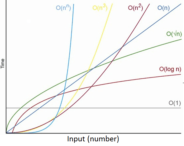
I’ll cover more detailed content like how to calculate Big O notation in another post.

Sorting Algorithms

Sorting algorithms are one of the important problems in computer science — given a dataset, the problem is to rearrange it in a specified order.

In real development, you’ll frequently encounter situations where you need to sort irregular data before searching through it. The key is whether you can effectively solve the problem by using the right algorithm for the situation.

For example, imagine you have a bag containing balls numbered 1 through 10 in random order, and you need to take them out one by one and arrange them from smallest to largest. Most humans can sort these without much difficulty. But computers often deal with 10,000 or even 10,000,000 pieces of data. And databases theoretically need to handle infinite amounts of data.

If the data isn’t sorted, you’d have to look at each piece of data sequentially while searching. But if the data is already sorted, you can use powerful algorithms like the binary search I mentioned above. (This is actually the biggest reason.)

Now let’s look at the representative sorting algorithms: bubble sort, selection sort, insertion sort, merge sort, and quick sort.

Bubble Sort

Bubble sort shows the worst performance in almost every situation, but it shows the best performance on already-sorted data since it only needs to traverse once. You might wonder why you’d sort already-sorted data, but it’s meaningful because the sorting algorithm itself operates without knowing whether the data is sorted or not.

Bubble sort works in the following order:

Compare and sort the 0th and 1st elements
Compare and sort the 1st and 2nd elements
…keep repeating
Compare and sort the (n-1)th and nth elements

Each traversal sorts one element at the end, so it looks like bubbles rising — hence the name bubble sort. The principle is intuitive and easy to implement, but it’s a fairly inefficient sorting method. So typically you implement it once when first learning, but I’ve rarely seen it used in practice.

Here’s the implementation code for bubble sort:

function bubbleSort<T>(input: T[]) {
  const len = input.length;
  let tmp: T | null = null;

  for (let i = 0; i < len; i++) {
    for (let j = 0; j < len; j++) {
      if (input[j] > input[j + 1]) {
        tmp = input[j];
        input[j] = input[j + 1];
        input[j + 1] = tmp;
        tmp = null;
      }
    }
  }

  return input;
}

Selection Sort

Selection sort is a sorting algorithm that finds and selects the appropriate data for the current position from the given data and swaps positions. After one traversal, the smallest value in the entire dataset will be at the 0th index according to the algorithm, so from the next traversal onward, you just repeat the process starting from index 1.

Selection sort works in the following order:

Find the smallest value from index 0 to n and swap it with index 0
Find the smallest value from index 1 to n and swap it with index 1
…keep repeating
Find the smallest value from index n-1 to n and swap it with index n

Selection sort traverses the entire list regardless of whether the current data is sorted or not, so it consistently has $O(n^2)$ time complexity in both best and worst cases. Here’s the implementation code for selection sort:

function selectionSort<T>(input: T[]) {
  const len = input.length;
  let tmp: T | null = null;

  for (let i = 0; i < len; i++) {
    for (let j = 0; j < len; j++) {
      if (input[i] < input[j]) {
        tmp = input[j];
        input[j] = input[i];
        input[i] = tmp;
        tmp = null;
      }
    }
  }

  return input;
}

Insertion Sort

Insertion sort compares each element from the given data, from the beginning, with the already-sorted portion and inserts it in its proper position. It’s actually the sorting method most similar to how humans naturally sort things. Imagine sorting cards in your hand — you’d probably do something like this:

Pick up a card.
Look through the cards you’re holding.
Insert the current card in the position where it belongs.

Insertion sort works similarly to this process:

Skip index 0.
Find where the value at index 1 should go among indices 0-1 and insert it
Find where the value at index 2 should go among indices 0-2 and insert it
…keep repeating
Find where the value at index n should go among indices 0-n and insert it

In the best case, insertion sort only needs to traverse the entire data once, giving it $O(n)$ time complexity, but in the worst case, it has $O(n^2)$ time complexity.

Here’s the implementation code for insertion sort:

function insertionSort<T>(input: T[]) {
  const len = input.length;

  for (let i = 1; i < len; i++) { // Start from the second card
    const value = input[i]; // Pick up the card
    let j = i-1;
    for (;j > -1 && input[j] > value; j--) {
      // Look at the already-sorted cards from the back
      // If the examined card is larger than the current card
      // Move the examined card back one position
      input[j+1] = input[j];
    }
    // After moving is done
    // Place the current card one position after
    // the card that's smaller than it
    input[j+1] = value;
  }

  return input;
}

Merge Sort

Merge sort is a type of divide and conquer algorithm — it breaks a big problem into several smaller problems, solves each one, and then combines the results to solve the original problem. As the name “merge” suggests, it’s an algorithm that sorts during the process of splitting the given data into small pieces and then merging them back together. Here’s how it works:

Receive data [5, 0, 4, 1]
Split the data list in half until each piece has length 1
Becomes [5, 0], [4, 1]
Becomes [5], [0], [4], [1]
Since each list now has length 1, start merging
Compare index 0 of left with index 0 of right, merge the smaller value first. Between [5] and [0], 0 is smaller, so merge 0 into the new list first
Create [0, 5]
Compare index 0 of left with index 0 of right, merge the smaller value first. Between [4] and [1], 1 is smaller, so merge 1 into the new list first
Create [1, 4]
Now merge [0, 5] and [1, 4]. Since these lists are sorted, smaller indices are guaranteed to have smaller values.
Compare index 0 of left with index 0 of right, merge the smaller value first
Create [0]. [5] and [1, 4] remain
Compare index 0 of left with index 0 of right, merge the smaller value first
Create [0, 1]. [5] and [4] remain
Compare index 0 of left with index 0 of right, merge the smaller value first
Create [0, 1, 4]. [5] remains
Since there’s a value left, just merge it
[0, 1, 4, 5] sorting complete

Looking at the emphasized Compare index 0 of left with index 0 of right, merge the smaller value first in the process above, you can see this step keeps repeating.

Because it keeps repeating and merging in the same way, merge sort is typically implemented using recursion. Also, merge sort always has $O({n\log n})$ time complexity, making it efficient. However, since it needs to split and separately store elements equal to the number of elements, it has $O(n)$ space complexity. In other words, it trades memory for execution speed.

Here’s the implementation code for merge sort:

function merge<T>(left: T[], right: T[]) {
  const result: (T | undefined)[] = [];

  while (left.length && right.length) {
    if (left[0] <= right[0]) {
      result.push(left.shift());
    }
    else {
      result.push(right.shift());
    }
  }

  while (left.length) {
    result.push(left.shift());
  }

  while(right.length) {
    result.push(right.shift());
  }

  return result as T[];
}

function mergeSort<T>(input: T[]): T[] {
  if (input.length < 2) {
    return input;
  }

  const middle = input.length / 2;
  const left = input.slice(0, middle);
  const right = input.slice(middle, input.length);

  return merge(mergeSort(left), mergeSort(right));
}

Quick Sort

Quick sort is also a divide and conquer sorting method like merge sort. The difference from merge sort is that merge sort does nothing during the division phase and performs sorting during the merge phase, while quick sort performs important operations during the division phase and does nothing during merging.

Here’s the execution order for quick sort:

Select one element from the input data list. This element is called the Pivot.
Divide the list in two based on the pivot.
Move all elements smaller than the pivot to the left of the pivot
Move all elements larger than the pivot to the right of the pivot

function quickSort(arr:number[], left: number, right: number) {
  if (left < right) {
    // Find the pivot point and classify smaller/larger numbers around it
    const i =  position(arr, left, right);
    // Sort left of pivot
    quickSort(arr, left, i - 1);
    // Sort right of pivot
    quickSort(arr, i + 1, right);
  }
  return arr;
}

function position(arr: number[], left: number, right: number) {
  let i = left;
  let j = right;
  const pivot = arr[left];

  // In-place arrangement of larger/smaller numbers to left/right
  while (i < j) {
    while (arr[j] > pivot) j--;
    while (i < j && arr[i] <= pivot) i++;

    const tmp = arr[i];
    arr[i] = arr[j];
    arr[j] = tmp;
  }

  arr[left] = arr[j];
  arr[j] = pivot;

  return j;
}

That wraps up this post on sorting algorithms.